Advanced Transmission Line Modeling Techniques …

1 Section : Advanced Transmission line Modeling TechniquesBy Martin J King, 07/05/02 Copyright 2002 by Martin J. King. All Rights 1 of 12 Section : Advanced Transmission line Modeling TechniquesIn Section , two simple models were derived for a closed end and an openend Transmission line . In both of these models the driver is located at one end of thetransmission line and the cross-sectional area is monotonically varied based on a taperratio m and the exponential area equation found in Section For a straight-linegeometry m = 0 and this is equivalent to the test line geometry shown in Figure withan open or a closed end boundary most Transmission line designs.

2 The driver is not all the way at one end of theline and the cross-sectional area is much more complicated with changes in areaoccurring at several locations along the line s length. To model these more complicatedenclosures, a second set of MathCad worksheets were formulated and are presented inthis the Driver in a Transmission line :To address the offset driver geometry, the MathCad model TL Open needed to be rewritten to reflect the situation shown in Figure When a driver isinstalled offset from the closed end of the Transmission line , the line is split into twoseparate sections.

3 Above the driver is typically a short Transmission line with a closedterminus. Below the driver is a longer Transmission line with an open terminus. Noticethat these two Transmission lines are in parallel as seen from the back of the equivalent acoustic circuit and equivalent electrical circuit for thetransmission line with an offset driver are shown in Figures and that in the equivalent acoustic circuit, the acoustic impedance of the closed lineand the acoustic impedance of the open line are in parallel.

4 Also notice the relationshipbetween the volume velocities at the back of the Figure , recognize that as the driver moves into the cabinet, the air volumedisplaced moves into the closed ended Transmission line and into the open endedtransmission line . The volume split will depend on the relative values of the two acousticimpedances Zac and Zao. Also notice that the volume velocity of the air at the terminus isno longer a function of the volume velocity of the driver. The volume velocity of the air atthe terminus is a function of the volume velocity of the air entering the open endedtransmission the first quarter wavelength mode, offsetting the driver has no significantimpact.

5 The most obvious impact of offsetting the driver in a Transmission line is a dip ornull in the terminus response. This shows up in both stuffed and unstuffed terminusresponses. In the frequencies above the first quarter wavelength resonance, thedramatic attenuation of the terminus output can locally reduce if not eliminate the rippletypically seen in most Transmission line system SPL responses. = Ud + UcUo = ULSL UoSoSection : Advanced Transmission line Modeling TechniquesBy Martin J King, 07/05/02 Copyright 2002 by Martin J.

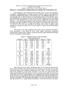
6 King. All Rights 2 of 12 The reason for the severe dip or null in the terminus response can be found inFigure for an unstuffed closed end Transmission line . In this figure the first halfwavelength mode is seen as a spike at 171 Hz. But at the frequency corresponding to aquarter wavelength standing wave, ~86 Hz, a deep null can be seen in the pressureresponse. Since the acoustic impedance of a Transmission line is the ratio of thepressure to the volume velocity, a deep null must also exist in the acoustic impedance ofthe closed end line .

7 A deep null in this acoustic impedance will tend to short the parallelimpedances in Figure and all of the driver s volume velocity will be directed into theclosed end. The means that the output from the terminus will be strongly a stuffed Transmission line , the same phenomenon can be observed. Thedamping from the fibrous tangle will tend to reduce the sharpness of all the resonantpeaks and at the same time reduce the depth of the first null resulting from the closedend portion of the Transmission line .

8 By reducing the sharpness of the peaks and nulls,the frequency content is also locally broadening for the volume velocities into the openand closed ends of the Transmission line . The resulting shallower dip will not attenuatethe terminus response as much as the unstuffed line but it will still have a significantlywider effect on the total SPL system summary, offsetting the driver from the end of a Transmission line willdramatically reduce the terminus SPL response at the quarter wavelength frequencies ofthe closed end section of the Transmission line .

9 By shifting the position of the driver, theposition of the dips in the terminus response can be moved higher or lower in geometry can be used to reduce the midrange ripple inherent in a Transmission linedesign with a driver mounted at one end. It should also be recognized that shifting thedriver does not change the basic quarter wavelength frequencies that would becalculated for the entire Transmission line length. Only the amount of excitation applied toeach quarter wavelength mode is the driver is offset to a location at approximately one third the length of astraight Transmission line , the 3/4 wavelength standing wave can be totally fact, the impact from every other quarter wavelength mode (3/4, 7/4, 11/4.)

10 Will beessentially removed from the system SPL MathCad worksheet TL Open was reconfigured to model theequivalent circuits in Figures and The third worksheet is called TL . This MathCad computer model can be used to simulate an offset driver, ina tapered, straight, or expanding fiber damped Transmission line . This model will handlea wide variety of geometries with Dacon Hollofil II stuffing densities between lb/ft3and lb/ft3. The only restriction on the geometry is that the closed end cross-sectionalarea Sc must be greater than zero.