Transcription of Air Pollution Modeling – An Overview
1 Daly, A. and P. Zannetti. 2007. Air Pollution Modeling An Overview . Chapter 2 of AMBIENT AIR Pollution (P. Zannetti, D. Al-Ajmi, and S. Al-Rashied, Editors). Published by The Arab School for Science and Technology (ASST) ( ) and The EnviroComp Institute ( ). Chapter 2 Air Pollution Modeling An Overview Aaron Daly and Paolo Zannetti The EnviroComp Institute, Fremont, CA (USA) and Abstract: This chapter presents a brief review of air Pollution Modeling techniques, , computer methods for the simulation of air quality processes. The review includes models developed or recommended by governmental agencies for regulatory applications. Both non-reactive ( , plume models) and reactive ( , photochemical models) are discussed. We also provide Web sites where the reader can download Modeling software. Key Words: Air Pollution , Computer Modeling , Eulerian and Lagrangian models, Gaussian models, puff models, photochemical models.
2 1 Introduction1 Air Pollution Modeling is a numerical tool used to describe the causal relationship between emissions, meteorology, atmospheric concentrations, deposition, and other factors. Air Pollution measurements give important, quantitative information about ambient concentrations and deposition, but they can only describe air quality at specific locations and times, without giving clear guidance on the identification of the causes of the air quality problem. Air Pollution Modeling , instead, can give a more complete deterministic description of the air quality problem, including an analysis of factors and causes (emission sources, meteorological processes, and 1 Builtjes, P. (2003) The Problem Air Pollution . Chapter 1 of AIR QUALITY Modeling Theories, Methodologies, Computational Techniques, and Available Databases and Software.)
3 Vol I Fundamentals (P. Zannetti, Editor). EnviroComp Institute ( ) and Air & Waste Management Association ( ). 2007 The Arab School for Science and Technology (ASST) and The EnviroComp Institute 15 16 Ambient Air Pollution physical and chemical changes), and some guidance on the implementation of mitigation measures. Air Pollution models play an important role in science, because of their capability to assess the relative importance of the relevant processes. Air Pollution models are the only method that quantifies the deterministic relationship between emissions and concentrations/depositions, including the consequences of past and future scenarios and the determination of the effectiveness of abatement strategies. This makes air Pollution models indispensable in regulatory, research, and forensic applications. The concentrations of substances in the atmosphere are determined by: 1) transport, 2) diffusion, 3) chemical transformation, and 4) ground deposition.
4 Transport phenomena, characterized by the mean velocity of the fluid, have been measured and studied for centuries. For example, the average wind has been studies by man for sailing purposes. The study of diffusion (turbulent motion) is more recent. Among the first articles that mention turbulence in the atmosphere, are those by Taylor (1915, 1921). 2 Modeling of Point Sources One of the first challenges in the history of air Pollution Modeling ( , Sutton, 1932, Bosanquet, 1936) was the understanding of the diffusion properties of plumes emitted from large industrial stacks. For this purpose, a very successful, yet simple model was developed the Gaussian Plume Model. This model was applied for the main purpose of calculating the maximum ground level impact of plumes and the distance of maximum impact from the source. The Gaussian plume model is illustrated in the figure below (Courtesy: Figure 19-5 of Boubel et al.)
5 , 1994). The model was formulated by determining experimentally the horizontal and vertical spread of the plume, measured by the standard deviation of the plume s spatial concentration distribution. 2 Air Pollution Modeling 17 Experiments provided the geometrical description of the plume by plotting the standard deviation of its concentration distribution, in both the vertical and horizontal direction, as a function of the atmospheric stability and downwind distance from the source. The plotting is presented in the figure below (Courtesy: Figure 19-6 of Boubel et al., 1994). Atmospheric stability is a parameter that characterizes the turbulent status of the atmosphere. This parameter ranges from very stable , class F, to neutral , class D, up to very unstable , class A. 18 Ambient Air Pollution The experimental sigma values discussed above are, in their functions with distance from the source, in reasonable agreement with the Taylor-theory.
6 The differences are caused by the fact that the Taylor-theory holds for homogeneous turbulence, which is not the exact case in the atmosphere. In the 1960s, the studies concerning dispersion from a point source continued and were broadening in scope. Major studies were performed by H gstrom (1964), Turner (1964), Briggs (1965) (the developer of the well-known plume-rise formulas), Moore (1967), Klug (1968). The use and application of the Gaussian plume model spread over the whole globe, and became a standard technique in every industrial country to calculate the stack height required for permits, see for example Beryland (1975) who published a standard work in Russian. The Gaussian plume model concept was soon applied also to line and area-sources. Gradually, the importance of the mixing height was realized (Holzworth, 1967, Deardorff, 1975) and its major influence on the magnitude of ground level concentrations.
7 To include the effects of the mixing height, multiple reflections terms were added to the Gaussian Plume model ( , Yamartino, 1977). 3 Air Pollution Modeling at Urban and Larger Scales Shortly after 1970, scientists began to realize that air Pollution was not only a local phenomenon. It became clear - firstly in Europe - that the SO2 and NOx emissions from tall stacks could lead to acidification at large distances from the sources. It also became clear - firstly in the US - that ozone was a problem in urbanized and industrialized areas. And so it was obvious that these situations could not be tackled by simple Gaussian-plume type Modeling . Two different Modeling approaches were followed, Lagrangian Modeling and Eulerian Modeling . In Lagrangian Modeling , an air parcel (or puff ) is followed along a trajectory, and is assumed to keep its identity during its path.
8 In Eulerian Modeling , the area under investigation is divided into grid cells, both in vertical and horizontal directions. Lagrangian Modeling , directed at the description of long-range transport of sulfur, began with studies by Rohde (1972, 1974), Eliassen (1975) and Fisher (1975). The work by Eliassen was the start for the well-known EMEP-trajectory model which has been used over the years to calculate trans-boundary air Pollution of acidifying species and later, photo-oxidants. Lagrangian Modeling is often used to cover longer periods of time, up to years. Eulerian Modeling began with studies by Reynolds (1973) for ozone in urbanized areas, with Shir and Shieh (1974) for SO2 in urban areas, and Egan (1976) and Carmichael (1979) for regional scale sulfur. From the Modeling studies by Reynolds on the Los Angeles basin, the well-known Urban Airshed Model-UAM 2 Air Pollution Modeling 19 originated for photochemical simulations.
9 Eulerian Modeling , in these years, was used only for specific episodes of a few days. So in general, Lagrangian Modeling was mostly performed in Europe, over large distances and longer time-periods, and focused primarily on SO2. Eulerian grid Modeling was predominantly applied in the US, over urban areas and restricted to episodic conditions, and focused primarily on O3. Also hybrid approaches were studied, as well as particle-in-cell methods (Sklarew et al., 1971). Early papers on both Eulerian and Lagrangian Modeling are by Friedlander and Seinfeld (1969), Eschenroeder and Martinez (1970) and Liu and Seinfeld (1974). A comprehensive Overview of long-range transport Modeling in the seventies was presented by Johnson (1980). The next, obvious step in scale is global Modeling of earth s troposphere. The first global models were 2-D models, in which the global troposphere was averaged in the longitudinal direction (see Isaksen, 1978).
10 The first, 3-D global models were developed by Peters (1979) (see also Zimmermann, 1988). It can be stated that, since approximately 1980, the basic Modeling concepts and tools were available to the scientific community. Developments after 1980 concerned the fine-tuning of these basic concepts. 4 Examples of Dispersion Models We present below some discussion on specific air computer models that are particularly important and are used by a large community of scientists. The US-EPA today recommends the following two computer packages for simulation of non-reactive chemicals ( , SO2): AERMOD: #aermod AERMOD is a steady-state Gaussian plume model. It uses a single wind field to transport emitted species. The wind field is derived from surface, upper-air, and onsite meteorological observations. AERMOD also combines geophysical data such as terrain elevations and land use with the meteorological data to derive boundary layer parameters such as Monin-Obukhov length, mixing height, stability class, turbulence, etc.