Transcription of Alternating Direction Method of Multipliers
1 Alternating Direction Method of MultipliersRyan TibshiraniConvex Optimization 10-725 Last time: dual ascentConsider the problemminxf(x) subject toAx=bwherefis strictly convex and closed. Denote LagrangianL(x,u) =f(x) +uT(Ax b)Dual gradient ascent repeats, fork= 1,2,3,..x(k)= argminxL(x,u(k 1))u(k)=u(k 1)+tk(Ax(k) b)Good:xupdate decomposes whenfdoes. Bad: require stringentassumptions (strong convexity off) to ensure convergence2 Augmented Lagrangian Method modifies the problem, for >0,minxf(x) + 2 Ax b 22subject toAx=buses a modified LagrangianL (x,u) =f(x) +uT(Ax b) + 2 Ax b 22and repeats, fork= 1,2,3,..x(k)= argminxL (x,u(k 1))u(k)=u(k 1)+ (Ax(k) b)Good: better convergence properties. Bad: lose decomposability3 Alternating Direction Method of multipliersAlternating Direction Method of Multipliers or ADMM tries for thebest of both methods. Consider a problem of the form:minx,zf(x) +g(z) subject toAx+Bz=cWe define augmented Lagrangian, for a parameter >0,L (x,z,u) =f(x) +g(z) +uT(Ax+Bz c) + 2 Ax+Bz c 22We repeat, fork= 1,2,3.
2 X(k)= argminxL (x,z(k 1),u(k 1))z(k)= argminzL (x(k),z,u(k 1))u(k)=u(k 1)+ (Ax(k)+Bz(k) c)4 Convergence guaranteesUnder modest assumptions onf,g(these do not requireA,Btobe full rank), the ADMM iterates satisfy, for any >0: Residual convergence:r(k)=Ax(k)+Bz(k) c 0ask , , primal iterates approach feasibility Objective convergence:f(x(k)) +g(z(k)) f?+g?, wheref?+g?is the optimal primal objective value Dual convergence:u(k) u?, whereu?is a dual solutionFor details, see Boyd et al. (2010). Note that we do not genericallyget primal convergence, but this is true under more assumptionsConvergence rate: roughly, ADMM behaves like first-order still being developed, see, , in Hong and Luo (2012),Deng and Yin (2012), Iutzeler et al. (2014), Nishihara et al. (2015)5 Scaled form ADMMS caled form: denotew=u/ , so augmented Lagrangian becomesL (x,z,w) =f(x) +g(z) + 2 Ax+Bz c+w 22 2 w 22and ADMM updates becomex(k)= argminxf(x) + 2 Ax+Bz(k 1) c+w(k 1) 22z(k)= argminzg(z) + 2 Ax(k)+Bz c+w(k 1) 22w(k)=w(k 1)+Ax(k)+Bz(k) cNote that herekth iteratew(k)is just a running sum of residuals:w(k)=w(0)+k i=1(Ax(i)+Bz(i) c)6 OutlineToday: Examples, practicalities Consensus ADMM Special decompositions7 Connection to proximal operatorsConsiderminxf(x) +g(x) minx,zf(x) +g(z) subject tox=zADMM steps (equivalent to Douglas-Rachford, here):x(k)= proxf,1/ (z(k 1) w(k 1))z(k)= proxg,1/ (x(k)+w(k 1))w(k)=w(k 1)+x(k) z(k)whereproxf,1/ is the proximal operator forfat parameter1/ ,and similarly forproxg,1/ In general, the update for block of variables reduces to prox updatewhenever the corresponding linear transformation is the identity8 Example: lasso regressionGiveny Rn,X Rn p, recall the lasso problem.
3 Min 12 y X 22+ 1We can rewrite this as:min , 12 y X 22+ 1subject to = 0 ADMM steps: (k)= (XTX+ I) 1(XTy+ ( (k 1) w(k 1))) (k)=S / ( (k)+w(k 1))w(k)=w(k 1)+ (k) (k)9 Notes: The matrixXTX+ Iis always invertible, regardless ofX If we compute a factorization (say Cholesky) inO(p3)flops,then each update takesO(p2)flops The update applies the soft-thresolding operatorSt, whichrecall is defined as[St(x)]j= xj t x > t0 t x txj+t x < t, j= 1,..,p ADMM steps are almost like repeated soft- thresholding ofridge regression coefficients10 Comparison of various algorithms for lasso regression: 100 randominstances withn= 200,p= 5001020304050601e 101e 071e 041e 01 Iteration kSuboptimality fk fstarCoordinate descProximal gradAccel proxADMM (rho=50)ADMM (rho=100)ADMM (rho=200)11 PracticalitiesIn practice, ADMM usually obtains a relatively accurate solution ina handful of iterations, but it requires a large number of iterationsfor a highly accurate solution (like a first-order Method )Choice of can greatly influence practical convergence of ADMM: too large not enough emphasis on minimizingf+g too small not enough emphasis on feasibilityBoyd et al.
4 (2010) give a strategy for varying ; it can work well inpractice, but does not have convergence guaranteesLike deriving duals, transforming a problem into one that ADMMcan handle is sometimes a bit subtle, since different forms can leadto different algorithms12 Example: group lasso regressionGiveny Rn,X Rn p, recall the group lasso problem:min 12 y X 22+ G g=1cg g 2 Rewrite as:min , 12 y X 22+ G g=1cg g 2subject to = 0 ADMM steps: (k)= (XTX+ I) 1(XTy+ ( (k 1) w(k 1))) (k)g=Rcg / ( (k)g+w(k 1)g), g= 1,..,Gw(k)=w(k 1)+ (k) (k)13 Notes: The matrixXTX+ Iis always invertible, regardless ofX If we compute a factorization (say Cholesky) inO(p3)flops,then each update takesO(p2)flops The update applies the group soft-thresolding operatorRt,which recall is defined asRt(x) =(1 t x 2)+x Similar ADMM steps follow for a sum of arbitrary norms of asregularizer, provided we know prox operator of each norm ADMM algorithm can be rederived when groups have overlap(hard problem to optimize in general!)
5 See Boyd et al. (2010)14 Example: sparse subspace estimationGivenS Sp(typicallyS 0is a covariance matrix), consider thesparse subspace estimation problem (Vu et al., 2013):maxYtr(SY) Y 1subject toY FkwhereFkis the Fantope of orderk, namelyFk={Y Sp: 0 Y I,tr(Y) =k}Note that when = 0, the above problem is equivalent to ordinaryprincipal component analysis (PCA)This above is an SDP and in principle solveable with interior-pointmethods, though these can be complicated to implement and quiteslow for large problem sizes15 Rewrite as:minY,Z tr(SY) +IFk(Y) + Z 1subject toY=ZADMM steps are:Y(k)=PFk(Z(k 1) W(k 1)+S/ )Z(k)=S / (Y(k)+W(k 1))W(k)=W(k 1)+Y(k) Z(k)HerePFkis Fantope projection operator, computed by clipping theeigendecompositionA=U UT, = diag( 1,.., p):PFk(A) =U UT, = diag( 1( ),.., p( ))where each i( ) = min{max{ i ,0},1}, and pi=1 i( ) =k16 Example: sparse + low rank decompositionGivenM Rn m, consider the sparse plus low rank decompositionproblem (Candes et al.)
6 , 2009):minL,S L tr+ S 1subject toL+S=MADMM steps:L(k)=Str1/ (M S(k 1)+W(k 1))S(k)=S`1 / (M L(k)+W(k 1))W(k)=W(k 1)+M L(k) S(k)where, to distinguish them, we useStr / for matrix soft-thresoldingandS`1 / for elementwise soft-thresolding17 Example from Candes et al. (2009):(a) Original frames(b) Low-rank L(c) Sparse S(d) Low-rank L(e) Sparse SConvex optimization (this work) Alternating minimization [47]Figure 2:Background modeling from video. Three frames from a 200 frame video sequencetaken in an airport [32]. (a) Frames of original videoM. (b)-(c) Low-rank Land sparsecomponents Sobtained by PCP, (d)-(e) competing approach based on Alternating minimizationof anm-estimator [47]. PCP yields a much more appealing result despite using less 2 (d) and (e) compares the result obtained by Principal Component Pursuit to a state-of-the-art technique from the computer vision literature, [47].12 That approach also aims at robustlyrecovering a good low-rank approximation, but uses a more complicated, nonconvexm-estimator,which incorporates a local scale estimate that implicitly exploits the spatial characteristics of naturalimages.
7 This leads to a highly nonconvex optimization, which is solved locally via alternatingminimization. Interestingly, despite using more prior information about the signal to be recovered,this approach does not perform as well as the convex programming heuristic: notice the largeartifacts in the top and bottom rows of Figure 2 (d).In Figure 3, we consider 250 frames of a sequence with several drastic illumination , the resolution is 168 120, and soMis a 20,160 250 matrix. For simplicity, and toillustrate the theoretical results obtained above, we again choose =1 this example,on the same GHz Core 2 Duo machine, the algorithm requires a total of 561 iterations and 36minutes to 3 (a) shows three frames taken from the original video, while (b) and (c) show therecovered low-rank and sparse components, respectively. Notice that the low-rank componentcorrectly identifies the main illuminations as background, while the sparse part corresponds to the12We use the code package downloaded ~ftorre/papers/ , modi-fied to choose the rank of the approximation as suggested in [47].
8 13 For this example, slightly more appealing results can actually be obtained by choosing larger (say, 2/pn1).2518 Consensus ADMMC onsider a problem of the form:minxB i=1fi(x)The consensus ADMM approach begins by reparametrizing:minx1,..,xB,xB i=1fi(xi) subject toxi=x, i= 1,..BThis yields the decomposable ADMM steps:x(k)i= argminxifi(xi) + 2 xi x(k 1)+w(k 1)i 22, i= 1,..,Bx(k)=1BB i=1(x(k)i+w(k 1)i)w(k)i=w(k 1)i+x(k)i x(k), i= 1,..,B19 Write x=1B Bi=1xiand similarly for other variables. Not hard tosee that w(k)= 0for all iterationsk 1 Hence ADMM steps can be simplified, by takingx(k)= x(k):x(k)i= argminxifi(xi) + 2 xi x(k 1)+w(k 1)i 22, i= 1,..,Bw(k)i=w(k 1)i+x(k)i x(k), i= 1,..,BTo reiterate, thexi,i= 1,..,Bupdates here are done in parallelIntuition: Try to minimize eachfi(xi), use (squared)`2regularization topull eachxitowards the average x If a variablexiis bigger than the average, thenwiis increased So the regularization in the next step pullsxieven closer20 General consensus ADMMC onsider a problem of the form:minxB i=1fi(aTix+bi) +g(x)For consensus ADMM, we again reparametrize:minx1.
9 ,xB,xB i=1fi(aTixi+bi) +g(x) subject toxi=x, i= 1,..BThis yields the decomposable ADMM updates:x(k)i= argminxifi(aTixi+bi) + 2 xi x(k 1)+w(k 1)i 22,i= 1,..,Bx(k)= argminxB 2 x x(k) w(k 1) 22+g(x)w(k)i=w(k 1)i+x(k)i x(k), i= 1,..,B21 Notes: It is no longer true that w(k)= 0at a general iterationk, soADMM steps do not simplify as before To reiterate, thexi,i= 1,..,Bupdates are done in parallel Eachxiupdate can be thought of as a loss minimization onpart of the data, with`2regularization Thexupdate is a proximal operation in regularizerg Thewupdate drives the individual variables into consensus A different initial reparametrization will give rise to a differentADMM algorithmSee Boyd et al. (2010), Parikh and Boyd (2013) for more detailson consensus ADMM, strategies for splitting up into subproblems,and implementation tips22 Special decompositionsADMM can exhibit much faster convergence than usual, when weparametrize subproblems in a special way ADMM updates relate closely to block coordinate descent, inwhich we optimize a criterion in an Alternating fashion acrossblocks of variables With this in mind, get fastest convergence when minimizingover blocks of variables leads to updates in nearly orthogonaldirections Suggests we should design ADMM form (auxiliary constraints)so that primal updates de-correlate as best as possible This is done in, , Ramdas and Tibshirani (2014), Wytocket al.
10 (2014), Barbero and Sra (2014)23 Example: 2d fused lassoGiven an imageY Rd d, equivalently written asy Rn, the 2dfused lasso or 2d total variation denoising problem is:min 12 Y 2F+ i,j(| i,j i+1,j|+| i,j i,j+1|) min 12 y 22+ D 1 HereD Rm nis a 2d difference operator giving the appropriatedifferences (across horizontally and vertically adjacent positions)164 Parallel and Distributed AlgorithmsFigure : Variables are black dots; the partitionsPandQare in orange and next step is to transform ( ) into the canonical form ( ):minimize Ni=1fi(xi)+IC(x1,..,xN),( )whereCis theconsensussetC={(x1,..,xN)|x1= =xN}.( )In this formulation we have moved the consensus constraint into theobjective using an indicator function. In the notation of ( ),fis thesum of the termsfi,whilegis the indicator function of the consistencyconstraint. The partitions are given byP={[n],n+[n],2n+[n],..,(N 1)n+[n]},Q={{i, n+i,2n+i, .. ,(N 1)n+i}|i=1,..,N}.The first partition is clear sincefis additive.