Transcription of An Introduction to statistics Survival Analysis 1
1 Introduction to statistics Survival Analysis 1 Robin Beaumont D:\web_sites_mine\HIcourseweb new\stats\statistics2\ page 1 of 22 McKelvey et al., 1976 Time (days ) % surviving, S(t)An Introduction to statistics Survival Analysis 1 Written by: Robin Beaumont e-mail: Date last updated Friday, 15 October 2010 Version: 1 This document has been designed to be suitable for both web based and face-to-face teaching. The text has been made to be as interactive as possible with exercises, Multiple Choice Questions (MCQs) and web based exercises. If you are using this document as part of a web-based course you are urged to use the online discussion board to discuss the issues raised and share your solutions with other students. This document is part of a series see: I hope you enjoy working through this document.
2 Robin Beaumont Acknowledgments My sincere thanks go to Claire Nickerson for not only proofreading several drafts but also providing additional material and technical advice. Also I must applaud the material available on the web from the medical statistician, Malcolm Farrow's course on Survival Analysis at ~nmf16/teaching/mas3311/ while he goes a lot further than this short Introduction it has provided some key information concerning how to use R in this context. 112 20112 2(++..)0( )( ) exp(++..)()()kkikkxxxit htxxxh t h te +=+= Hazard at time t = i Baseline hazard 's = Relative risks =hazard ratios (HR) Hazard = death rate = Kaplan Meier product-limit (PL) graph Cox Regression Introduction to statistics Survival Analysis 1 Robin Beaumont D:\web_sites_mine\HIcourseweb new\stats\statistics2\ page 2 of 22 Contents 1.
3 Introduction .. 3 2. GRAPHING THE Survival FUNCTION THE K-M PLOT .. 3 PRODUCING A K-P PLOT IN R .. 5 3. SEVERAL CURVES .. 6 Descriptive statistics .. 7 COMPARING CURVES THE LOGRANK AND BESLOW statistics .. 8 4. THE COX REGRESSION MODEL .. 9 The null model for comparison ..11 5. USING SPSS ..12 6. INTERPRETING THE BETA'S ( ) ..12 7. HAZARD RATIOS, ODDS AND PROBABILITIES ..13 8. FINDING INDIVIDUAL HR SCORES ..13 9. ASSUMPTIONS, DANGERS AND ASSESSMENT OF COX 10. MULTIPLE CHOICE QUESTIONS ..15 11. EXERCISES ..17 12. SUMMARY ..19 13. 14. APPENDIX R CODE ..21 Introduction to statistics Survival Analysis 1 Robin Beaumont D:\web_sites_mine\HIcourseweb new\stats\statistics2\ page 3 of 22 1. Introduction Survival Analysis is concerned with looking at how long it takes to an event to happen of some sort.
4 The event is usually something that you do not want to happen such as failure, however it might be a positive thing such as 'recovery' or healing or a specific treatment state such as remission. Campbell 2009 provides the example of an exercise stress test where the event is the point at which the subject cannot carry on any longer on the machine. Fortunately or unfortunately depending upon the 'event', some subjects never reach it during the course of the study and in which case they are said to be censored. This can be for several reasons and there are actually different types of censoring (see Lee & Wang 2003 , Cox & Oates 1984 ), the subject might be lost to follow up, or the study time might be relatively short, or if the event is reliant upon equipment for example in the exercise stress test, the equipment might fail so in effect the subject has no event in that instance and is censored.
5 The degree of censoring can affect the reliability of the results and there are recommendations for the maximum % of censoring allowable in a group along with sample size. For many years Analysis of such data needed the help of a statistician and a mainframe computer. When I undertook Survival Analysis of various types of renal patient in the late 1980's I needed to use a mainframe computer and a very unfriendly statistical package called BMDP, this has now all changed and you can now easily carry out complex analyses of Survival data on your laptop. Survival Analysis has become a major area of medical statistical research with the UK leading the way, with one of the most widely used and influential models being the Cox regression model developed by professor D R Cox at Oxford University in the 1970's ( (statistician).)
6 Several UK medical schools run courses on Survival Analysis , such as the excellent one by Malcolm Farrow at Newcastle medical school ( ~nmf16/teaching/mas3311/ ). These are much more advanced than the material I intend to cover here but I have made use of much web material particularly that from Malcolm's site. Why do we need to consider the Analysis of ' Survival ' data differently from other data, well there are two reasons, the Censored nature of a proportion of the data and also the fact that it does not tend to follow a normal distribution, you may remember in the chapter on measuring spread we looked a waiting times and realised how they tended to follow an exponential distribution ( ). The easiest way to get some understanding of what an Analysis of Survival data entails is to consider how you might graph a typical dataset.
7 The most common type of graph is the Kaplan Meier product-limit (PL) graph which estimates the Survival function S(t) against time. 2. Graphing the Survival function the K-M plot The following are a set of Survival times (in days from entry to a trial) for patients with stage 3 diffuse hystiocytic lymphoma (from McKelvey, Gottlieb 1976, Cancer, 38, 1484-1493). The graph on the right is the Kaplan Meier product-limit (PL) graph of the data, commonly called the K-M plot, the vertical dashes represent the censored items, showing how the majority of them are at the far right of the graph as would be expected. In the table on the right I indicates the status (1=completed;0=censored) for each subject, alternatively often censored observations are indicated by a star, asterisk or + symbol.
8 Notice that in our dataset 8 out of the 19 observations are not censored representing 50%. This is usually a good quick check to ensure you have used the censored / uncensored values the right way round, as the censored observations Survival time (weeks) 1= completed 0=censored 6 1 19 1 32 1 42 1 42 1 43 0 94 1 126 0 169 0 207 1 211 0 227 0 253 1 255 0 270 0 310 0 316 0 335 0 346 0 [ ] McKelvey et al., 1976 Time (days ) % surviving, S(t) Introduction to statistics Survival Analysis 1 Robin Beaumont D:\web_sites_mine\HIcourseweb new\stats\statistics2\ page 4 of 22 do not affect the % surviving. Unfortunately 50% does not help matters much here as coding either way we will end up with a line at 50%, subsequent examples demonstrate this more successfully. Obviously the effective sample size decreases as we move from the left to the right of the K-M plot and this affects the accuracy of the estimates.
9 Some authors provide a table along the bottom of the x axis or a separate one indicating the number of non-censored observations at several time points. Obviously, the lines on the K -M plot relate to a set of x,y values and investigating how these are calculated provides insight into what S(t) means, that is the values on the y axis. The table below shows how this is carried out. First lets consider some points of nomenclature. i = A time point, numbered on ordered Survival times, from 0 to p, where p is equal to the number of cases/observations, there may be duplicate times (Machin, Campbell & Walters 2007 ) they will rarely be equal. di = Number of cases failing at time ti ni = Number at risk just before time i [notice the downward pointing arrows in table below] ri= Number alive just before time i (ni-di)/ni = proportion surviving interval i =probability of surviving i [notice the horizontal arrows in table below] S(t) = probability of surviving from start (i=0) to ti = cumulative Survival probability = Kaplan Meier Product limit estimator Failure time Ranked from shortest to largest, then uncensored,censored I di = No.
10 Failing at time ti ni = no. at risk ri= no. alive just before i (ni-di)/ni =proportion surviving interval i =probability of surviving i S(t) = probability of surviving from start (i=0) to ti = cumulative Survival probability = Kaplan Meier Product limit estimator 0 0 - 19 - 1 6 1 1 19 (19-1)/19= 19 2 1 19-1=18 (18-1)/18= 32 3 1 18-1=17 (17-1)17= 42 4 2 17-1=16 (16-2)/16= 43* 5 0 16-2=14 1 94 6 1 16-3=13 (13-1)/13 126* 7 0 12 1 169* 8 0 11 1 207 9 1 11-1=10 (10-1)/10 211* 10 0 9 1 227* 11 0 8 1 253 12 1 8-1=7 (7-1)/7 There are three important aspects to note about the above: The proportion surviving in the penultimate column relates to the current Survival time i it is a conditional probability (Norman & Streiner 2008 ) The S(t) function relates to all time intervals up to time i The failure time ti is a value not an interval.