Transcription of ANALYSIS OF CONTINUOUS VARIABLES …
1 ANALYSIS OF CONTINUOUS VARIABLES / 31. CHAPTER SIX. ANALYSIS OF CONTINUOUS VARIABLES : comparing MEANS. In the last chapter, we addressed the ANALYSIS of discrete VARIABLES . Much of the statistical ANALYSIS in medical research, however, involves the ANALYSIS of CONTINUOUS VARIABLES (such as cardiac output, blood pressure, and heart rate) which can assume an infinite range of values. As with discrete VARIABLES , the statistical ANALYSIS of CONTINUOUS VARIABLES requires the application of specialized tests. In general, these tests compare the means of two (or more) data sets to determine whether the data sets differ significantly from one another. There are four situations in biostatistics where we might wish to compare the means of two or more data sets.
2 Each situation requires a different statistical test depending on whether the data is normally or non-normally distributed about the mean (Figure 6-1). 1. When we wish to compare the observed mean of a data set with a standard or normal value, we use the test of hypothesis or the sign test. 2. When we wish to determine whether the mean in a single patient group has changed as a result of a treatment or intervention, the single-sample, paired t-test or Wilcoxon signed- ranks test is appropriate. 3. When we are evaluating the means of two different groups of patients, we use the two- sample, unpaired t-test or Wilcoxon rank-sum test. 4. When multiple comparisons are required to determine how one therapy differs from several others, we employ ANALYSIS of variance (ANOVA).
3 The use of multiple comparisons is discussed in the next chapter. If we wish to compare: Normally Distributed Non-Normally Distributed Data Data A mean with a normal value Test of Hypothesis Sign Test Paired observations within a Single-sample, paired t-test Wilcoxon signed-ranks test single patient group Means from two different Two-sample, unpaired t-test Wilcoxon rank-sum test patient groups Nonparametric Multiple patient groups ANOVA. ANOVA. Figure 6-1: ANALYSIS of CONTINUOUS VARIABLES comparing MEANS. There are three factors which determine whether an observed sample mean is different from another mean or normal value. First, the larger the difference between the means, the more likely the difference has not occurred by chance. Second, the smaller the variability in the data about the mean, the more likely the observed sample mean represents the true mean of the population-at-large.
4 The standard deviation represents the variability of the data about the mean. The smaller the standard deviation, the smaller the variability of the data about the mean. Third, the larger the sample size, the more accurately the sample mean will represent the true population mean. The standard error of the mean estimates how closely the sample mean approximates the true population mean. As the sample size increases (and approaches the size of the population), the standard error of the mean approaches zero. 32 / A PRACTICAL GUIDE TO BIOSTATISTICS. THE t DISTRIBUTION: ANALYSIS OF NORMALLY DISTRIBUTED DATA. The t distribution is a probability distribution which is frequently used to evaluate hypotheses regarding the means of CONTINUOUS VARIABLES . It is commonly referred to as "Student's t-test" after William Gosset, a mathematician with the Guinness Brewery, who in 1908 noted that if one samples a normally distributed bell-shaped population, the sample observations will also be normally distributed (assuming the sample size is greater than 30).
5 Unfortunately, company policy forbade employee publishing and he was forced to use the pseudonym "Student." He named the distribution, "t", and defined a measure of the difference between two means known as the "critical ratio" or "t statistic". which followed the t distribution: x- x- . t= =. se sd / n where x = the mean of the sample observations, = the mean of the population , and se = the standard error of the sample mean (which is equal to the sample standard deviation divided by the square root of the sample size, n). The t distribution is similar to the standard normal (z) distribution (discussed in Chapter Two) in that it is symmetrically distributed about a mean of zero. Unlike the normal distribution, however, which has a standard deviation of 1, the standard deviation of the t distribution varies with an entity known as the degrees of freedom.
6 Since the t-test plays a prominent role in many statistical calculations, degrees of freedom is an important statistical concept. Degrees of freedom is related to sample size and indicates the number of observations in a data set that are free to vary. For example, if we make n observations and calculate their mean, we are free to change only n - 1 of the observations if the mean is to remain the same as once we have done so, we will automatically know the value of the nth observation. The degrees of freedom for a data set are therefore equal to the sample size (n) - 1. Whereas there is only one standard normal (z) distribution, there is a separate t distribution for each possible degree of freedom from 1 to . As with the normal distribution, critical values of the t-statistic can be obtained from t distribution tables (found in any statistics textbook) based on the desired significance level (p-value) and the degrees of freedom.
7 Appropriate use of the t distribution requires that three assumptions are met. The first assumption is that the observations follow a normal (gaussian or "bell-shaped") distribution; that is, they are evenly distributed about the true population mean. If the observations are not normally distributed, the t-statistic is not accurate and should not be used. As a general rule, if the median differs markedly from the mean, the t-test should not be used. The second assumption is that the variances (the standard deviations squared) of the two groups being compared, although unknown, are equal. The third assumption is that the observations occur independently ( , an observation in one group does not influence the occurrence of an observation in the other group).
8 THE t DISTRIBUTION AND CONFIDENCE INTERVALS. In Chapter Three, we saw that confidence intervals could be calculated for any mean in order to evaluate how confident we were that our sample mean represented the true population mean. In order to calculate the 95% confidence interval for a mean we used the following equation: 95% confidence interval = mean approximately 2 se Remember that this calculated the approximate confidence interval. In reality, the exact multiplying factor for the standard error of the mean depends on the sample size and degrees of freedom. Using the t distribution, we can calculate the exact 95% confidence interval for a particular mean (x) and standard deviation (sd) as follows (the critical value of t is obtained from a t distribution table based on the desired significance level and degrees of freedom present): sd 95% confidence interval = x t se = x t.
9 N For example, suppose we studied 87 intensive care unit (ICU) patients and found that the mean ICU. LOS (length of stay) was days with a standard deviation of days. If we wish to determine how ANALYSIS OF CONTINUOUS VARIABLES / 33. closely our observed mean ICU LOS approximates the true mean LOS for all ICU patients with 95%. confidence, we would determine the critical value of t for a significance level of (5% chance of a Type I error) and 86 (87-1) degrees of freedom. The critical value of t for these parameters, as obtained from a t distribution table, is Calculating the confidence interval as above we obtain: 95% confidence interval = = days 87. Therefore, we can be 95% confident that, based on our study data, the interval from to days contains the true mean LOS for all ICU patients.
10 ANALYSIS OF NORMALLY DISTRIBUTED CONTINUOUS VARIABLES . The t-test is commonly used in statistical ANALYSIS . It is an appropriate method for comparing two groups of CONTINUOUS data which are both normally distributed. The most commonly used forms of the t- test are the test of hypothesis, the single-sample, paired t-test, and the two-sample, unpaired t-test. TEST OF HYPOTHESIS. Suppose we know from previous experience that the normal mean LOS for all ICU patients in our hospital is days and we wish to compare this to our study mean of days to determine whether these two means differ significantly. To do so, we would use a form of the t-test known as the test of hypothesis in which we compare a single observed mean with a standard or normal value.