Applying Q-Learning to Flappy Bird

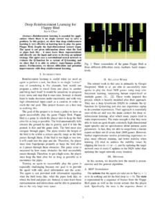
1 Applying Q-Learning to Flappy Bird Moritz Ebeling-Rump, Manfred Kao, Zachary Hervieux-Moore Abstract The field of machine learning is an interesting and bird is a two-dimensional side-scrolling game, illustrated in relatively new area of research in artificial intelligence. In this Figure 1, featuring retro style graphics. The goal of the game paper, a special type of reinforcement learning, Q-Learning , is to direct the bird through a series of pipes. If the bird was applied to the popular mobile game Flappy Bird. The Q- Learning algorithm was tested on two different environments. touches the floor or a pipe, then the bird will die and the game The original version and a simplified version. The maximum restarts. The only action that players are able to perform is score achieved on the original version and simplified version to make the bird jump. Otherwise, the bird will fall due were 169 and 28,851, respectively.

2 The trade-off between run- to gravity. Each pipe the bird successfully clears, the score time and accuracy was investigated. Using appropriate settings, is incremented. In the original game, the gap between the the Q-Learning algorithm was proven to be successful with a relatively quick convergence time. pipes are held constant but the height of the gap is uniformly distributed. In the simplified version that was considered, the I. INTRODUCTION height of the gap is held constant. The game is meant to test Q-Learning is form a reinforcement learning that players' endurance as there is no end to the game. does not require the agents to have prior knowledge of the environment dynamics [1]. The agents do not have II. THEORY. access to the cost function or the transition probabilities. Watkins and Dayan first showed convergence of the Q- Reinforcement learning is a type of learning strategy where Learning algorithm in [1].

3 However, Tsitsiklis gives an the agents are not told which actions to take. Instead, the alternate proof of convergence with stronger results in [6]. It agents discovers which action yields the highest reward is Tsitsiklis's results that will be shown here. To begin, define from experimentation [2]. Q-Learning was first introduced the standard form of a stochastic approximation algorithms. by Watkins in 1989 [3] and it was not until 1992 that the convergence was shown by Watkins and Dayan [1]. xi := xi + i (Fi (x) xi + i ) (1). Where x = (x1 , x2 , .., xn ) Rn , F1 , F2 , .., Fn are mappings from Rn R, i is a noise term, and i is the step size. Assumptions on equations of this form are now listed. Note, in Tsitsiklis's paper, he allows for outdated information. For simplicity, it is assumed all information available to the controller is up to date which will simplify ths list.

4 This is justified as the application considered has a controller that never uses outdated information. Assumption 1: (a) x(0) is F (0)-measurable. (b) i and t, wi is F (t + 1)-measurable. (c) i and t, i (t) is F (t)-measurable. (d) i and t, we have E[ i (t)|F (t)] = 0. (e) constants A and B such that E[ i2 (t)|F (t)] A + B max max |xj ( )|2 , i, t j t Assumption 1 is the typical restrictions imposed on stochastic systems. First, the present can be determined entirely by previous information. Second, the noise term has mean 0. and bounded variance. Fig. 1. The gameplay of Flappy Bird Assumption 2: (a) i, Flappy Bird is a mobile game developed in 2013 by Dong . Nyugen [4] and published by dotGears, a small independent X. i (t) = , 1. game developer company based in Vietnam [5]. Flappy t=0. (b) C such that i, when F (x) is written in this form, it can be shown that.

5 X Assumptions 1 and 4 are met. Hence, by Theorem 3, we i (t)2 C, 1 only need Assumption 2 for convergence to be guaranteed. t=0 This is an assumption on the step size so it is very easy Assumption 2 are restrictions on the step size to ensure that it for the algorithm user to impose this restriction in practice. approaches 0 at a slow enough speed to ensure convergence For our application, we will rewrite this cost minimization of the algorithm. as a reward maximization and use different notation as The following conventions are now used. If x y then shorthand: xi yi i. The norm k kv is defined as: h i |xi | F (Qt (st , at )) = E [Rt+1 ] + E max Qt (st+1 , a). kxkv = max , x Rn a i vi We now start with the Q-Learning algorithm and work our Assumption 3: way backwards to the stochastic approximation algorithm in (a) The mapping F is monotone. That is, if x y then equation 1.

6 F (x) F (y). (b) The mapping F is continuous. Qt+1 (st , at ) = Qt (st , at ) + t (st , at ) . (c) The mapping F has a unique fixed point x . n o Rt+1 + max Qt (st+1 , a) Qt (st , at ). (d) If e Rn is the vector whose components are all equal a to 1, and r > 0, then, = Qt (st , at ) + t (st , at ) . {Rt+1 + E [Rt+1 ] E [Rt+1 ]. F (X) re F (x re) F (x + re) F (X) + re h i h i It is not hard to imagine how Assumption 3 might be used + E max Qt (st+1 , a) E max Qt (st+1 , a) |It a a to generate inequalities that are essential in a proof. o + max Qt (st+1 , a) Qt (st , at ) , Assumption 4: a vector x Rn , a positive vector v, a and a [0, 1) such that, where It denotes the information available to the controller at time t. kF (x) x kv kx x kv , x Rn It can be seen that the previous assumption provides the and framework for a contraction argument (since [0, 1)).]]}

7 Wt (st , at ) =Rt+1 E [Rt+1 ] + max Qt (st+1 , a). a This can be used to prove convergence to a stationary point. h i E max Qt (st+1 , a) |It . a Assumption 5: a positive vector v, and a [0, 1) and Rewriting the expression for Q we get D such that, Qt+1 (st , at ) = Qt (st , at ) + t (st , at ) . kF (x)kv kxkv + D, x Rn (F (Qt (st , at )) Qt (st , at ) + wt (st , at )). Tsitsiklis goes on the prove the following three theorems. Theorem 1: Let Assumptions 1,2, and 5 hold. Then, then Q is now in the desired form! Thus, we only need to sequence x(t) in the stochastic approximation is bounded impose the restictions on (t) to guarantee convergence of with probability 1. Q. The last case we wish to consider is when the problem Theorem 2: Let Assumptions 1,2, and 3 hold. Then, then is undiscounted ( = 1). For this, one further assumption is sequence x(t) in the stochastic approximation is bounded needed.]

8 With probability 1. Assumption 6: Theorem 3: Let Assumptions 1,2, and 4 hold. Then, then (a) at least one proper stationary policy sequence x(t) in the stochastic approximation converges to (b) Every improper stationary policy yields infinite expected x with probability 1. cost for at least one initial state From these theorems, it is clear that Theorem 3 is the Where a proper policy is defined to be a stationary policy strongest in the sense that we need the fewest assumptions to that the probability of going to an absorbing state with 0. guarantee convergence. Also, Theorem 2 requires bounded- reward converges to 1. Otherwise, it is improper. With this, ness which is the result of Theorem 1. Thus, one can think of we get the last theorem: these as: to guarantee convergence, one needs Assumptions Theorem 4: The Q-Learning algorithm converges with 1, 2, 4, and 5 or 1, 2, and 3.

9 Probability 1 if we impose Assumption 2 and: With regards to Q-Learning , the way these theorems are (a) < 1, important depends on writing F (x) as follows: (b) = 1, Qiu (0) = 0, and all policies are proper, or (c) = 1, Qiu (0) = 0, Assumption 6 holds, and Q(t) is Fiu (Q) = E[ciu ] + min Qs(i,u),v guaranteed to be bounded with probability 1. v U (s(t,u)). III. IMPLEMENTATION exact values of the reward function are not as important as The key to a successful implementation of Q-Learning is long as reinforcement is positive and punishment is negative. modeling the problem efficiently. As long as the state space We weigh the benefit of survival lower than the punishment is finite, Q-Learning will converge. In practical applications, of death, as the goal is to avoid death. (. we are looking to obtain results in a limited time frame. 15, if bird alive If the state space is very large, the algorithm will take too Rt+1 =.)

10 1000, if bird dead long to converge. On the other hand, if the state space is very small, accuracy will be lost. Thus, there is a trade-off The learning rate determines to what extent new informa- between run-time and accuracy. tion overrides old information. The following learning was The dimension of the state space will be kept to a minimum chosen: by only considering three attributes: 1. t (st , at ) = Pt X distance from the next pipe 1 + k=0 1{sk =st ,ak =at }. Y distance from the next pipe Life of the bird The discount factor determines the importance of future rewards. This value is given below. A visual representation of the first two attributes are shown in Figure 2 = 1. These are the essential definitions that are needed to imple- ment the Q-Learning algorithm. Now the Q-Learning pseudocode that we used in our imple- mentation is shown below. 1) Initialize Q matrix 2) Repeat a) Determine the action, a, in state, s, based on Q matrix b) Take the action, a, and observe the outcome state, s, and reward, r c) Update Q matrix based on Equation 2.