Transcription of Chapter 11 Nonlinear Optimization Examples
1 Chapter 11 Nonlinear Optimization ExamplesChapter Table of ..307 Kuhn-Tucker Conditions ..308 Definition of Return ..319 Termination Criteria..325 ControlParametersVector ..332 PrintingtheOptimizationHistory ..334 Nonlinear Optimization Chemical ..343 example MLEs for Two-Parameter Weibull Profile-Likelihood-Based Confidence ..357 example A Two-Equation Maximum Likelihood Problem ..363 example Time-Optimal Heat Conduction .. Chapter 11. Nonlinear Optimization ExamplesSAS OnlineDoc : Version 8 Chapter 11 Nonlinear Optimization ExamplesOverviewThe IML procedure offers a set of Optimization subroutines for minimizing or max-imizing a continuous Nonlinear functionf=f(x)ofnparameters, wherex=(x1;:::;xn)T. The parameters can be subject to boundary constraints and linearor Nonlinear equality and inequality constraints. The following set of optimizationsubroutines is available:NLPCGC onjugate Gradient MethodNLPDDD ouble Dogleg MethodNLPNMSN elder-Mead Simplex MethodNLPNRAN ewton-Raphson MethodNLPNRRN ewton-Raphson Ridge MethodNLPQN(Dual) Quasi-Newton MethodNLPQUAQ uadratic Optimization MethodNLPTRT rust-Region MethodThe following subroutines are provided for solving Nonlinear least-squares problems.
2 NLPLML evenberg-Marquardt Least-Squares MethodNLPHQNH ybrid Quasi-Newton Least-Squares MethodsA least-squares problem is a special form of minimization problem where the objec-tive function is defined as a sum of squares of other ( Nonlinear ) (x)=12ff21(x)+ +f2m(x)gLeast-squares problems can usually be solved more efficiently by the least-squaressubroutines than by the other Optimization following subroutines are provided for the related problems of computing finitedifference approximations for first- and second-order derivatives and of determininga feasible point subject to boundary and linear constraints:NLPFDDA pproximate Derivatives by Finite DifferencesNLPFEAF easible Point Subject to ConstraintsEach Optimization subroutine works iteratively. If the parameters are subject onlyto linear constraints, all Optimization and least-squares techniques arefeasible-pointmethods; that is, they move from feasible pointx(k)to a better feasible pointx(k+1)by a step in the search directions(k),k=1;2;3.
3 If you do not provide a feasiblestarting pointx(0), the Optimization methods call the algorithm used in the NLPFEA subroutine, which tries to compute a starting point that is feasible with respect to theboundary and linear Chapter 11. Nonlinear Optimization ExamplesThe NLPNMS and NLPQN subroutines permit Nonlinear constraints on problems with Nonlinear constraints, these subroutines do not use a feasible-point method; instead, the algorithms begin with whatever starting point you specify,whether feasible or Optimization technique requires a continuous objective functionf=f(x)andall Optimization subroutines except the NLPNMS subroutine require continuous first-order derivatives of the objective functionf. If you do not provide the derivatives off, they are approximated by finite difference formulas. You can use the NLPFDD subroutine to check the correctness of analytical derivative of the results obtained from the IML procedure Optimization and least-squaressubroutines can also be obtained by using the NLP procedure in the SAS/OR advantages of the IML procedure are as follows: You can use matrix algebra to specify the objective function, Nonlinear con-straints, and their derivatives in IML modules.
4 The IML procedure offers several subroutines that can be used to specify theobjective function or Nonlinear constraints, many of which would be very dif-ficult to write for the NLP procedure. You can formulate your own termination criteria by using the"ptit" advantages of the NLP procedure are as follows: Although identical Optimization algorithms are used, the NLP procedure canbe much faster because of the interactive and more general nature of the IMLproduct. Analytic first- and second-order derivatives can be computed with a specialcompiler. Additional Optimization methods are available in the NLP procedure that donot fit into the framework of this package. Data set processing is much easier than in the IML procedure. You can saveresults in output data sets and use them in following runs. The printed output contains more OnlineDoc : Version 8 Getting Started 299 Getting StartedUnconstrained Rosenbrock FunctionThe Rosenbrock function is defined asf(x)=12f100(x2 x21)2+(1 x1)2g=12ff21(x)+f22(x)g;x=(x1;x2)The minimum function valuef =f(x )=0is at the pointx =(1;1).
5 The following code calls the NLPTR subroutine to solve the Optimization problem:proc iml;title Test of NLPTR subroutine: Gradient Specified ;start F_ROSEN(x);y1 = 10. * (x[2] - x[1] * x[1]);y2 = 1. - x[1];f = .5 * (y1 * y1 + y2 * y2);return(f);finish F_ROSEN;start G_ROSEN(x);g = j(1,2,0.);g[1] = -200.*x[1]*(x[2]-x[1]*x[1]) - ( [1]);g[2] = 100.*(x[2]-x[1]*x[1]);return(g);finish G_ROSEN;x = { 1.};optn = {0 2};call nlptr(rc,xres,"F_ROSEN",x,optn) grd="G_ROSEN";quit;The NLPTR is a trust-region Optimization method. The F ROSEN module repre-sents the Rosenbrock function, and the G ROSEN module represents its the gradient can reduce the number of function calls by the optimizationsubroutine. The Optimization begins at the initial pointx=( 1:2;1).Formoreinformation on the NLPTR subroutine and its arguments, see the section NLPTRCall on page 667. For details on the options vector, which is given by the OPTN vector in the preceding code, see the section Options Vector on page portion of the output produced by the NLPTR subroutine is shown in Figure page OnlineDoc : Version 8300 Chapter 11.
6 Nonlinear Optimization ExamplesTrust Region OptimizationWithout Parameter ScalingCRP Jacobian Computed by Finite DifferencesParameter Estimates 2 Optimization StartActive Constraints 0 Objective Function Abs Gradient Radius 1 ElementMax Abs TrustRest Func Act Objective Obj Fun Gradient RegionIter arts Calls Con Function Change Element Lambda Radius1 0 2 0 0 0 5 0 0 8 0 0 0 31 0 0 ResultsIterations 22 Function Calls 32 Hessian Calls 23 Active Constraints 0 Objective Function Max Abs Gradient 0 Actual Over Pred 0 ChangeRadius convergence criterion ResultsParameter EstimatesGradientObjectiveN Parameter Estimate Function1 X1 X2 of Objective Function = Solution to the Rosenbrock ProblemSincef(x)=12ff21(x)+f22(x)g, you can also use least-squares techniques in thissituation.
7 The following code calls the NLPLM subroutine to solve the problem. Theoutput is shown in Figure??on page??.proc iml;title Test of NLPLM subroutine: No Derivatives ;start F_ROSEN(x);y = j(1,2,0.);y[1] = 10. * (x[2] - x[1] * x[1]);y[2] = 1. - x[1];return(y);SAS OnlineDoc : Version 8 Getting Started 301finish F_ROSEN;x = { 1.};optn = {2 2};call nlplm(rc,xres,"F_ROSEN",x,optn);quit;The Levenberg-Marquardt least-squares method, which is the method used by theNLPLM subroutine, is a modification of the trust-region method for Nonlinear least-squares problems. The F ROSEN module represents the Rosenbrock function. Notethat for least-squares problems, themfunctionsf1(x);:::;fm(x)are specified aselements of a vector; this is different from the manner in whichf(x)is specifiedfor the other Optimization techniques. No derivatives are specified in the precedingcode, so the NLPLM subroutine computes finite difference approximations.
8 For moreinformation on the NLPLM subroutine, see the section NLPLM Call on page Betts FunctionThe linearly constrained Betts function (Hock & Schittkowski 1981) is defined asf(x)=0:01x21+x22 100with boundary constraints2 x1 50 50 x2 50and linear constraint10x1 x2 10 The following code calls the NLPCG subroutine to solve the Optimization infeasible initial pointx0=( 1; 1)is specified, and a portion of the output isshown in Figure iml;title Test of NLPCG subroutine: No Derivatives ;start F_BETTS(x);f = .01 * x[1] * x[1] + x[2] * x[2] - 100.;return(f);finish F_BETTS;con = { 2. -50..,50. 50..,10. -1. 1. 10.};x = {-1. -1.};optn = {0 2};call nlpcg(rc,xres,"F_BETTS",x,optn,con);quit ;SAS OnlineDoc : Version 8302 Chapter 11. Nonlinear Optimization ExamplesThe NLPCG subroutine performs conjugate gradient Optimization . It requires onlyfunction and gradient calls. The F BETTS module represents the Betts function,and since no module is defined to specify the gradient, first-order derivatives arecomputed by finite difference approximations.
9 For more information on the NLPCG subroutine, see the section NLPCG Call on page 634. For details on the constraintmatrix, which is represented by the CON matrix in the preceding code, see the section Parameter Constraints on page : Initial point was changed to be feasible for boundary andlinear StartParameter EstimatesGradient LowerObjective BoundN Parameter Estimate Function Constraint1 X1 X2 StartParameter of Objective Function = Constraints1 : <= + * X1 - * X2 Conjugate-Gradient OptimizationAutomatic Restart Update (Powell, 1977; Beale, 1972)Gradient Computed by Finite DifferencesParameter Estimates 2 Lower Bounds 2 Upper Bounds 2 Linear Constraints 1 Figure Solution to Betts ProblemSAS OnlineDoc.
10 Version 8 Getting Started 303 Optimization StartActive Constraints 0 Objective Function Abs Gradient 2 ElementMax Abs SlopeRest Func Act Objective Obj Fun Gradient Step SearchIter arts Calls Con Function Change Element Size Direc1 0 3 0 1 7 1 2 9 1 0 -74E-7 Optimization ResultsIterations 3 Function Calls 10 Gradient Calls 9 Active Constraints 1 Objective Function Max Abs Gradient 0 ElementSlope of Search convergence criterion ResultsParameter EstimatesGradient ActiveObjective BoundN Parameter Estimate Function Constraint1 X1 Lower BC2 X2 0 Value of Objective Function = Constraints Evaluated at Solution[1] = + * X1 - * X2 Figure (continued)Since the initial point( 1; 1)is infeasible, the subroutine first computes a feasiblestarting point.