Transcription of CHAPTER 21
1 801. CHAPTER . 21. The GPLOT Procedure Overview 801. About Plots of Two Variables 802. About Plots with a Classification Variable 803. About Bubble Plots 803. About Plots with Two Vertical Axes 804. About Interpolation Methods 805. Concepts 805. Parts of a Plot 805. About the Input Data Set 806. Missing Values 807. Values Out of Range 807. Sorted Data 807. Logarithmic Axes 807. Procedure Syntax 807. PROC GPLOT Statement 808. BUBBLE Statement 809. BUBBLE2 Statement 815. PLOT Statement 818. PLOT2 Statement 828. Examples 834. Example 1: Generating a Simple Bubble Plot 834. Example 2: Labeling and Sizing Plot Bubbles 835. Example 3: Adding a Right Vertical Axis 837. Example 4: Plotting Two Variables 839. Example 5: Connecting Plot Data Points 842. Example 6: Generating an Overlay Plot 844. Example 7: Filling Areas in an Overlay Plot 846.
2 Example 8: Plotting Three Variables 847. Example 9: Plotting with Different Scales of Values 851. Example 10: Creating Plots with Drill-down for the Web 853. Overview The GPLOT procedure plots the values of two or more variables on a set of coordinate axes (X and Y). The coordinates of each point on the plot correspond to two variable values in an observation of the input data set. The procedure can also generate a separate plot for each value of a third (classification) variable. It can also generate bubble plots in which circles of varying proportions representing the values of a third variable are drawn at the data points. The procedure produces a variety of two-dimensional graphs including 802 About Plots of Two Variables 4 CHAPTER 21. 3 simple scatter plots 3 overlay plots in which multiple sets of data points display on one set of axes 3 plots against a second vertical axis 3 bubble plots 3 logarithmic plots (controlled by the AXIS statement).
3 In conjunction with the SYMBOL statement the GPLOT procedure can produce join plots, high-low plots, needle plots, and plots with simple or spline-interpolated lines. The SYMBOL statement can also display regression lines on scatter plots. The GPLOT procedure is useful for 3 displaying long series of data, showing trends and patterns 3 interpolating between data points 3 extrapolating beyond existing data with the display of regression lines and confidence limits. About Plots of Two Variables Plots of two variables display the values of two variables as data points on one horizontal axis (X) and one vertical axis (Y). Each pair of X and Y values forms a data point. Figure on page 802 shows a simple scatter plot that plots the values of the variable HEIGHT on the vertical axis and the variable WEIGHT on the horizontal axis. By default, the PLOT statement scales the axes to include the maximum and minimum data values and displays a plus sign (+) at each data point.
4 It labels each axis with the name of its variable or an associated label and displays the value of each major tick mark. Figure Scatter Plot of Two Variables (GR21N04(a)). The program for this plot is in Example 4 on page 839. For more information on producing scatter plots, see PLOT Statement on page 818. The GPLOT Procedure 4 About Bubble Plots 803. You can also overlay two or more plots (multiple sets of data points) on a single set of axes and you can apply a variety of interpolation techniques to these plots. See About Interpolation Methods on page 805. About Plots with a Classi cation Variable Plots that use a classification variable produce a separate set of data points for each unique value of the classification variable and display all sets of data points on one set of axes. Figure on page 803 shows multiple line plots that compare yearly temperature trends for three cities.
5 The legend explains the values of the classification variable, CITY. Figure Plot of Three Variables with Legend (GR21N08(a)). By default, plots with a classification variable generate a legend. In the code that generates the plot for Figure on page 803, a SYMBOL statement connects the data points and specifies the plot symbol that is used for each value of the classification variable (CITY). The program for this plot is in Example 8 on page 847. For more information on how to produce plots with a classification variable, see PLOT. Statement on page 818. About Bubble Plots Bubble plots represent the values of three variables by drawing circles of varying sizes at points that are plotted on the vertical and horizontal axes. Two of the variables determine the location of the data points, while the values of the third variable control the size of the circles.
6 Figure on page 804 shows a bubble plot in which each bubble represents a category of engineer that is shown on the horizontal axis. The location of each bubble in relation to the vertical axis is determined by the average salary for the category. The size of each bubble represents the number of engineers in the category relative to the total number of engineers in the data. By default, the BUBBLE statement scales the axes to include the maximum and minimum data values and draws an unlabeled circle at each data point. It labels each 804 About Plots with Two Vertical Axes 4 CHAPTER 21. axis with the name of its variable or an associated label and displays the value of each major tick mark. Figure Bubble Plot (GR21N01). The program for this plot is in Example 1 on page 834. For more information on producing bubble plots, see BUBBLE Statement on page 809.
7 About Plots with Two Vertical Axes Plots with two vertical axes have a right vertical axis that can 3 display the same variable values as the left axis 3 display left axis values in a different scale 3 plot a second dependent (Y) variable, thereby producing one or more overlay plots. In Figure on page 805 the right axis displays the values of the vertical coordinates in a different scale from the scale that is used for the left axis. The GPLOT Procedure 4 Parts of a Plot 805. Figure Plot with a Right Vertical Axis (GR21N09). The program for this plot is in Example 9 on page 851. For more information on how to produce plots with a right vertical axis, see PLOT2 Statement on page 828 and BUBBLE2 Statement on page 815. About Interpolation Methods In addition to these graphs, you can produce other types of plots such as box plots or high-low-close plots by specifying various interpolation methods with the SYMBOL.
8 Statement. Use the SYMBOL statement to 3 connect the data points with straight lines 3 specify regression analysis to fit a line to the points and, optionally, display lines for confidence limits 3 connect the data points to the zero line on the vertical axis 3 display the minimum and maximum values of Y at each X value and mark the mean value, display standard deviations that connect the data points with lines or bars, generate box plots, or plot high-low-close stock market data 3 specify that a pattern fill the polygon that is defined by data points 3 smooth plot lines with spline interpolation 3 use a step function to connect the data points SYMBOL Statement on page 226 describes all interpolation methods. Concepts Parts of a Plot Some terms used with GPLOT procedure are illustrated in Figure on page 806. and Figure on page 806.
9 806 About the Input Data Set 4 CHAPTER 21. Figure GPLOT Procedure Terms Figure Additional GPLOT Procedure Terms About the Input Data Set The input data set that is used by the GPLOT procedure must contain at least one variable to plot on the horizontal axis and one variable to plot on the vertical axis. Typically, the horizontal axis shows an independent variable (time, for example), and the vertical axis shows a dependent variable (temperature, for example). Variables can The GPLOT Procedure 4 Procedure Syntax 807. be character or numeric. Graphs are automatically scaled to the values of the character data or to include the values of numeric data, but you can control scaling with procedure options or with associated AXIS statements. Missing Values If the value of either of the plot variables is missing, the GPLOT procedure does not include the observation in the plot.
10 If you specify interpolation with a SYMBOL. definition, the plot is not broken at the missing value. To break the plot line or area fill at the missing value, use the PLOT statement's SKIPMISS option. SKIPMISS is available only with join or spline interpolations. Values Out of Range Exclude data values from a graph by restricting the range of axis values with the VAXIS= or HAXIS= options or with the ORDER= option in an AXIS statement. When an observation contains a value outside of the specified axis range, the GPLOT. procedure excludes the observation from the plot and issues a message to the log. If you specify interpolation with a SYMBOL definition, by default values outside of the axis range are excluded from interpolation calculations and as a result may change interpolated values for the plot. Values that are omitted from interpolation calculations have a particularly noticeable effect on the high-low interpolation methods: HILO, STD, and BOX.