Transcription of Chapter 12 Bayesian Inference - Carnegie Mellon University
1 Chapter 12 Bayesian InferenceThis Chapter covers the following topics: Concepts and methods of Bayesian Inference . Bayesian hypothesis testing and model comparison. Derivation of the Bayesian information criterion (BIC). Simulation methods and Markov chain Monte Carlo (MCMC). Bayesian computation via variational Inference . Some subtle issues related to Bayesian What is Bayesian Inference ?There are two main approaches to statistical machine learning:frequentist(or classical)methods andBayesianmethods. Most of the methods we have discussed so far are fre-quentist. It is important to understand both approaches. At the risk of oversimplifying, thedifference is this:Frequentist versus Bayesian Methods In frequentist Inference , probabilities are interpreted as long run goal is to create procedures with long run frequency guarantees. In Bayesian Inference , probabilities are interpreted as subjective degrees of be-lief.
2 The goal is to state and analyze your Machine LearningCHAPTER INFERENCESome differences between the frequentist and Bayesian approaches are as follows:FrequentistBayesianProbability is:limiting relative frequency degree of beliefParameter is a:fixed constantrandom variableProbability statements are about:proceduresparametersFrequency guarantees?yesnoTo illustrate the difference, consider the following example. Suppose thatX1,..,Xn N( ,1). We want to provide some sort of interval estimateCfor .Frequentist the confidence intervalC= Xn ,Xn+ .ThenP ( 2C)= all probability statement is about the random intervalC. The interval is random becauseit is a function of the data. The parameter is a fixed, unknown quantity. The statementmeans thatCwill trap the true value with make the meaning clearer, suppose we repeat this experiment many times. In fact, wecan even allow to change every time we do the experiment.
3 The experiment looks likethis:Naturechooses 1 !Nature generatesndata points fromN( 1,1) !Statistician computesconfidence intervalC1 Naturechooses 2 !Nature generatesndata points fromN( 2,1) !Statistician computesconfidence will find that the intervalCjtraps the parameter j, 95 percent of the time. Moreprecisely,lim infn!11nnXi=1I( i2Ci) ( )almost surely, for any sequence 1, 2,.. Bayesian Bayesian treats probability as beliefs, not frequencies. Theunknown parameter is given a prior distributon ( )representing his subjective beliefs300 Statistical Machine Learning, by Han Liu and Larry Wasserman, c 2014 Statistical Machine WHAT IS Bayesian Inference ?about . After seeing the dataX1,..,Xn, he computes the posterior distribution for given the data using Bayes theorem: ( |X1,..,Xn)/L( ) ( )( )whereL( )is the likelihood function. Next we finds an intervalCsuch thatZC ( |X1,..,Xn)d = can thn report thatP( 2C|X1.)
4 ,Xn)= is a degree-of-belief probablity statement about given the data. It is not the sameas ( ). If we repeated this experient many times, the intervals wouldnottrap the truevalue 95 percent of the Inference is aimed at given procedures with frequency guarantees. Bayesianinference is about stating and manipulating subjective beliefs. In general, these are differ-ent, A lot of confusion would be avoided if we usedF(C)to denote frequency probablityandB(C)to denote degree-of-belief probability. These are idfferent things and there isno reason to expect them to be the same. Unfortunately, it is traditional to use the samesymbol, such asP, to denote both types of probability which leads to summarize: Frequentist Inference gives procedures with frequency probability guar-antees. Bayesian Inference is a method for stating and updating beliefs. A frequentistconfidence intervalCsatisfiesinf P ( 2C)=1 where the probability refers to random intervalC.
5 We callinf P ( 2C)the coverage ofthe intervalC. A Bayesian confidence intervalCsatisfiesP( 2C|X1,..,Xn)=1 where the probability refers to . Later, we will give concrete examples where the coverageand the posterior probability are very are, in fact, many flavors of Bayesian Inference . Subjective Bayesians in-terpret probability strictly as personal degrees of belief. Objective Bayesians try to findprior distributions that formally express ignorance with the hope that the resulting poste-rior is, in some sense, objective. Empirical Bayesians estimate the prior distribution fromthe data. Frequentist Bayesians are those who use Bayesian methods only when the re-sulting posterior has good frequency behavior. Thus, the distinction between Bayesian andfrequentist Inference can be somewhat murky. This has led to much confusion in statistics,machine learning and Machine Learning, by Han Liu and Larry Wasserman, c 2014301 Statistical Machine LearningCHAPTER Basic ConceptsLetX1.
6 ,Xnbenobservations sampled from a probability densityp(x| ). In this Chapter ,we writep(x| )if we view as a random variable andp(x| )represents the conditionalprobability density ofXconditioned on . In contrast, we writep (x)if we view as adeterministic The Mechanics of Bayesian InferenceBayesian Inference is usually carried out in the following choose a probability density ( ) called the prior distribution thatexpresses our beliefs about a parameter before we see any choose a statistical modelp(x| )that reflects our beliefs aboutxgiven . observing dataDn={X1,..,Xn}, we update our beliefs and calculatethe posterior distributionp( |Dn).By Bayes theorem, the posterior distribution can be written asp( |X1,..,Xn)=p(X1,..,Xn| ) ( )p(X1,..,Xn)=Ln( ) ( )cn/Ln( ) ( )( )whereLn( )=Qni=1p(Xi| )is the likelihood function andcn=p(X1,..,Xn)=Zp(X1,..,Xn| ) ( )d =ZLn( ) ( )d is the normalizing constant, which is also called the can get a Bayesian point estimate by summarizing the center of the posterior.
7 Typically,we use the mean or mode of the posterior distribution. The posterior mean is n=Z p( |Dn)d =Z Ln( ) ( )d ZLn( ) ( )d .302 Statistical Machine Learning, by Han Liu and Larry Wasserman, c 2014 Statistical Machine BASIC CONCEPTSWe can also obtain a Bayesian interval estimate. For example, for 2(0,1), we could findaandbsuch thatZa 1p( |Dn)d =Z1bp( |Dn)d = (a, b). ThenP( 2C|Dn)=Zbap( |Dn)d =1 ,soCis a1 Bayesian posterior interval or credible interval. If has more than onedimension, the extension is straightforward and we obtain a credible {X1,..,Xn}whereX1,..,Xn Bernoulli( ). Suppose we takethe uniform distribution ( )=1as a prior. By Bayes theorem, the posterior isp( |Dn)/ ( )Ln( )= Sn(1 )n Sn= Sn+1 1(1 )n Sn+1 1whereSn=Pni=1 Xiis the number of successes. Recall that a random variable on theinterval(0,1)has a Beta distribution with parameters and if its density is , ( )= ( + ) ( ) ( ) 1(1 ) see that the posterior distribution for is a Beta distribution with parametersSn+1andn Sn+1.
8 That is,p( |Dn)= (n+2) (Sn+1) (n Sn+1) (Sn+1) 1(1 )(n Sn+1) write this as |Dn Beta(Sn+1,n Sn+1).Notice that we have figured out the normalizing constant without actually doing the inte-gralZLn( ) ( )d . Since a density function integrates to one, we see thatZ10 Sn(1 )n Sn= (Sn+1) (n Sn+1) (n+2).The mean of aBeta( , )distribution is /( + )so the Bayes posterior estimator is =Sn+1n+ is instructive to rewrite as = nb +(1 n)e Statistical Machine Learning, by Han Liu and Larry Wasserman, c 2014303 Statistical Machine LearningCHAPTER Inference whereb =Sn/nis the maximum likelihood estimate,e =1/2is the prior mean and n=n/(n+2) 1. A 95 percent posterior interval can be obtained by numerically findingaandbsuch thatZbap( |Dn)d =. that instead of a uniform prior, we use the prior Beta( , ). If you repeat thecalculations above, you will see that |Dn Beta( +Sn, +n Sn). The flat prior is justthe special case with = =1.
9 The posterior mean in this more general case is = +Sn + +n= n + +n b + + + +n 0where 0= /( + )is the prior illustration of this example is shown in We use the Bernoulli model togeneraten=15data with parameter = We observes=7. Therefore, the maximumlikelihood estimate isb =7/15 = , which is larger than the true parameter left plot of a priorBeta(4,6)which gives a posterior mode ,while the right plot of a priorBeta(4,2)which gives a posterior : Illustration of Bayesian Inference on Bernoulli data with two priors. Thethree curves are prior distribution (red-solid), likelihood function (blue-dashed), and theposterior distribution (black-dashed). The true parameter value = indicated by thevertical Multinomial(n, )where =( 1,.., K)Tbe aK-dimensionalparameter (K>1). The multinomial model with a Dirichlet prior is a generalization ofthe Bernoulli model and Beta prior of the previous example.
10 The Dirichlet distribution for304 Statistical Machine Learning, by Han Liu and Larry Wasserman, c 2014 Statistical Machine BASIC CONCEPTSK outcomes is the exponential family distribution on theK 1dimensional probabilitysimplex1 Kgiven by ( )= (PKj=1 j)QKj=1 ( j)KYj=1 j 1jwhere =( 1,.., K)T2RK+is a non-negative vector of scaling coefficients, which arethe parameters of the model. We can think of the sample space of the multinomial withKoutcomes as the set of vertices of theK-dimensional hypercubeHK, made up of vectorswith exactly one1and the remaining elements0:x=(0,0,..,0,1,0,..,0)T|{z} (Xi1,..,XiK)T2HK. If Dirichlet( )andXi| Multinomial( )fori=1,2,..,n,then the posterior satisfiesp( |X1,..,Xn)/Ln( ) ( )/nYi=1 KYj=1 XijjKYj=1 j 1j=KYj=1 Pni=1 Xij+ j see that the posterior is also a Dirichlet distribution: |X1,..,Xn Dirichlet( +nX)whereX=n 1 Pni=1Xi2 the mean of a Dirichlet distribution ( )is given byE( )= 1 PKi=1 i.