Transcription of Chapter 3 Continuous Random Variables
1 Chapter 3 Continuous Random IntroductionRather thansummingprobabilities related to discrete Random Variables , here forcontinuous Random Variables , thedensitycurve isintegratedto determine (Introduction)Patient s number of visits,X, and duration of visit, =value of function,F(3) = P(Y < 3) = 5/12x , pmf f(x)probability (distribution): cdf F(x)probability less than = sum of probabilityat specific valuesP(X < ) = P(X = 0) + P(X = 1)= + = (X = 2) = , pdf f(y) = y/6, 2 < y < 4probability less than 3 = area under curve,P(Y < 3) = 5/12xprobability at 3,P(Y = 3) = 0probability less than = value of functionF( ) = P(X < ) = : Comparing discrete and Continuous distributions7374 Chapter 3. Continuous Random Variables (LECTURE NOTES 5)1.
2 Number of visits,Xis a (i)discrete(ii)continuousrandom variable,and duration of visit,Yis a (i)discrete(ii)continuousrandom (a)P(X= 2) = (i)0(ii) (iii) (iv) (b)P(X ) =P(X 1) =F(1) = + = (i)summation(ii)integrationand is a value of a(i)probability mass function(ii)cumulative distribution functionwhich is a (i)stepwise(ii)smooth increasingfunction(c)E(X) = (i) xf(x)(ii) xf(x)dx(d)V ar(X) = (i)E(X2) 2(ii)E(Y2) 2(e)M(t) = (i)E(etX)(ii)E(etY)(f) Examples of discrete densities (distributions) include (choose one or more)(i)uniform(ii)geometric(iii)hyperge ometric(iv)binomial (Bernoulli)(v) (a)P(Y= 3) = (i)0(ii) (iii) (iv) (b)P(Y 3) =F(3) = 32x6dx=x212]x=3x=2=3212 2212=512requires (i)summation(ii)integrationand is a value of a(i)probability density function(ii)cumulative distribution func-tionwhich is a (i)stepwise(ii)smooth increasingfunction(c)E(Y) = (i) yf(y)(ii) yf(y)dy(d)V ar(Y) = (i)E(X2) 2(ii)E(Y2) 2(e)M(t) = (i)E(etX)(ii)E(etY)(f) Examples of Continuous densities (distributions) include (choose one ormore)(i)uniform(ii)exponential(iii)nor mal (Gaussian)(iv)Gamma(v)chi-square(vi)stud ent-t(vii)FSection 2.
3 Definitions (LECTURE NOTES 5) DefinitionsRandom variableXiscontinuousifprobability density function(pdf)fis continuousat all but a finite number of points and possesses the following properties: f(x) 0, for allx, f(x)dx= 1, P(a < X b) = baf(x)dxThe(cumulative) distribution function(cdf) for Random variableXisF(x) =P(X x) = x f(t)dt,and has properties limx F(x) = 0, limx F(x) = 1, ifx1< x2, thenF(x1) F(x2); that is,Fis nondecreasing, P(a X b) =P(X b) P(X a) =F(b) F(a) = baf(x)dx, F (x) =ddx x f(t)dt=f(x).xacdf F(a) = P(X < a)density, f(x)abf(x) is positiveP(a < X < b) = F(b) - F(a)total area = 1_probability_probabilityFigure : Continuous distributionTheexpected valueormeanof Random variableXis given by =E(X) = xf(x)dx,thevarianceis 2=V ar(X) =E[(X )2] =E(X2) [E(X)]2=E(X2) 276 Chapter 3.
4 Continuous Random Variables (LECTURE NOTES 5)with associatedstandard deviation, = functionisM(t) =E[etX]= etXf(x)dxfor values oftfor which this integral value, assuming it exists, of a functionuofXisE[u(X)] = u(x)f(x)dxThe (100p)thpercentileis a value ofXdenoted pwherep= p f(x)dx=F( p)and where pis also called thequantile of order p. The 25th, 50th, 75th percentilesare also calledfirst,second,third quartiles, denotedp1= ,p2= ,p3= also 50th percentile is called themedianand denotedm=p2. Themodeis thevaluexwherefis (Definitions) the time waiting in line, in minutes, be described by the Random variableXwhich has the following pdf,f(x) ={16x,2< x 4,0, 1 231/31/22/3140 1 , cdf F(x)density, pdf f(x)probability less than 3 = area under curve,P(X < 3) = 5/12probability =value of function,F(3) = P(X < 3) = 5/12xxprobability at 3,P(X = 3) = 0 Figure : f(x) and F(x)Section 2.}
5 Definitions (LECTURE NOTES 5)77(a) Verify functionf(x) satisfies the second property of pdfs, f(x)dx= 4216x dx=x212]x=4x=2=4212 2212=1212=(i)0(ii) (iii) (iv)1(b)P(2< X 3) = 3216x dx=x212]x=3x=2=3212 2212=(i)0(ii)512(iii)912(iv)1(c)P(X= 3) =P(3 < X 3) =3212 3212= 06=f(3) =16 3 = (i)True(ii)FalseSo the pdff(x) =16xdetermined at some value ofxdoesnotdetermine probability.(d)P(2< X 3) =P(2< X <3) =P(2 X 3) =P(2 X <3)(i)True(ii)FalsebecauseP(X= 3) = 0 andP(X= 2) = 0(e)P(0< X 3) = 3216x dx=x212]x=3x=2=3212 2212=(i)0(ii)512(iii)912(iv)1 Why integrate from 2 to 3 and not 0 to 3?(f)P(X 3) = 3216x dx=x212]x=3x=2=3212 2212=(i)0(ii)512(iii)912(iv)1(g) determine cdf (not pdf)F(3).F(3) =P(X 3) = 3216x dx=x212]x=3x=2=3212 2212=(i)0(ii)512(iii)912(iv)1(h) DetermineF(3) F(2).
6 F(3) F(2) =P(X 3) P(X 2) =P(2 X 3) = 3216x dx=x212]x=3x=2=3212 2212=(i)0(ii)512(iii)912(iv)1because everything left of (below) 3 subtract everything left of 2 equals what is between 2 and 378 Chapter 3. Continuous Random Variables (LECTURE NOTES 5)(i) Thegeneraldistribution function (cdf) isF(x) = x 0dt= 0,x 2, x2t6dt=t212]t=xt=2=x212 412,2< x 4,1,x > other words,F(x) =x212 412=x2 412on (2,4]. Both pdf density and cdfdistribution are given in the figure above.(i)True(ii)False(j)F(2) =2212 412= (i)0(ii)512(iii)912(iv)1.(k)F(3) =3212 412= (i)0(ii)512(iii)912(iv)1.(l)P( < X < ) =F( ) F( ) =( 412) ( 412)=(i)0(ii) (iii) (iv)1.(m)P(X > ) = 1 P(X ) = 1 F( ) = 1 ( 412)=(i) (ii) (iii) (iv)1.(n)Expected average wait time is =E(X) = xf(x)dx= 42x(16x)dx= 42x26dx=x318]42=4318 2318=(i)239(ii)289(iii)319(iv) (MASS) # INSTALL once, RUN once (per session) library MASS mean <- 4^3/18 - 2^3/18; mean; fractions(mean) # turn decimal to fraction[1] [1] 28/9(o)Expected value of functionu= (X2)= x2f(x)dx= 42x2(16x)dx= 42x36dx=x424]42=4424 2424=(i)9(ii)10(iii)11(iv)12.)
7 (p)Variance, method in wait time is 2=V ar(X) =E(X2) 2= 10 (289)2=(i)2381(ii)2681(iii)3181(iv) (MASS) # INSTALL once, RUN once (per session) library MASS sigma2 <- 10 - (28/9)^2 ; fractions(sigma2) # turn decimal to fractionSection 2. Definitions (LECTURE NOTES 5)79[1] 26/81(q)Variance, method in wait time is 2=V ar(X) =E[(X )2] = (x )2f(x)dx= 42(x 289)2(16x)dx= 42(x36 56x254+784x486)dx=x424 56x3162+784x2972]42=(i)2381(ii)2681(iii) 3181(iv) (MASS) # INSTALL once, RUN once (per session) library MASS sigma2 <- (4^4/24 - 56*4^3/162 + 784*4^2/972) - (2^4/24 - 56*2^3/162 + 784*2^2/972)fractions(sigma2) # turn decimal to fraction[1] 26/81(r)Standard deviation in time spent on the call is, = 2= 2681 (i) (ii) (iii) (iv) (s)Moment generating (t) =E[etX] = etxf(x)dx= 42etx(16x)dx=16 42xetxdx=16etx(xt 1t2)]4x=2=16e4t(4t 1t2) 16e2t(2t 1t2), t6= 0.
8 (i)True(ii)Falseuse integration by parts fort6= 0 case: u dv=uv v duwhereu=x,dv= 3. Continuous Random Variables (LECTURE NOTES 5)(t) the distribution functionF(x) =x2 412, then medianm= whenF(m) =P(X m) =m2 412=12som= 122+ 4 (i) (ii) (iii) answerm is not in 2< x 4, som6= with thatf(x) ={ax2,1< x 5,0, 1 1 , cdf F(x) = P(X < x)density, pdf f(x)xxFigure : f(x) and F(x)(a)Find constanta. Since the cdfF(5) = 1, andF(x) = x1at2dt=at33]t=xt=1=ax33 a3=a(x3 1)3thenF(5) =a(53 1)3=124a3= 1,soa= (i)3124(ii)2124(iii)1124(b) determine (x) =ax2=(i)3124x2(ii)2124x2(iii)1124x2 Section 2. Definitions (LECTURE NOTES 5)81(c) determine (x) =a(x3 1)3=3124 x3 13=(i)3124(x3 1)(ii)2124(x3 1)(iii)1124(x3 1)(d) DetermineP(X 2).P(X 2) = 1 P(X <2) = 1 F(2) = 1 1124(23 1) =(i)61124(ii)117124(iii)61117(e) DetermineP(X 4).}
9 P(X 4) = 1 P(X <4) = 1 F(4) = 1 1124(43 1) =(i)61124(ii)117124(iii)61117(f) DetermineP(X 4|X 2).P(X 4|X 2) =P(X 4 X 2)P(X 2)=P(X 4)P(X 2)=61/124117/124=(i)116124(ii)117124(iii )61117(g)Expected value. =E(X) = xf(x)dx= 51x(3124x2)dx= 513x3124dx=3x4496]51=3 54496 3 14496=(i)11431(ii)11531(iii)11631(iv)117 31.(h)Expected value of functionu= (X2) = x2f(x)dx= 51x2(3124x2)dx= 513x4124dx=3x5620]51=3 55620 3 15620 (i) (ii) (iii) (iv) (i) determine 25th percentile (first quartile),p1= (x) =1124(x3 1), then,F( ) =1124( 1) = =14,and so 1244+ 1 (i) (ii) (iii) that value where 25% of probability is at or below (to the left of) this 3. Continuous Random Variables (LECTURE NOTES 5)(j) determine ( ) =1124( 1) = ,and so 124 + 1 (i) (ii) (iii) that value where 1% of probability is at or below (to the left of) this Random variableXhave pdff(x) = x,0< x 1,2 x,1< x 2,0, , cdf F(x) = P(X < x)density, pdf f(x)xxFigure : f(x) and F(x)(a)Expected value.
10 =E(X) = xf(x)dx= 10x(x)dx+ 21x(2 x)dx= 10x2dx+ 21(2x x2)dx=[x33]10+[2x22 x33]21=(133 033)+(22 233) (12 133)=(i)1(ii)2(iii)3(iv) 2. Definitions (LECTURE NOTES 5)83(b)E(X2).E(X2)= 10x2(x)dx+ 21x2(2 x)dx= 10x3dx+ 21(2x2 x3)dx=[x44]10+[2x33 x44]21=(144 044)+(2(2)33 244) (2(1)33 144)=(i)46(ii)56(iii)66(iv)76.(c)Varianc e. 2= Var(X) =E(X2) 2=76 12=(i)13(ii)14(iii)15(iv)16.(d)Standard deviation. = 2= 16 (i) (ii) (iii) (iv) (e) the distribution function isF(x) = 0x 0 x0t dt=t22]xt=0=x22,0< x 1, x1(2 t)dt+F(1) = 2t t22]xt=1+12= 2x x22 (2(1) 122) +12,1< x 2,1,x > (1) =12, so add12toF(x) for 1< x 2then medianmoccurs whenF(x) = m22=12,0< x 1,2m m22 1 =12,1< x 2,1,x > for both 0< x 1 and 1< x 2,m= (i)1(ii) (iii)284 Chapter 3. Continuous Random Variables (LECTURE NOTES 5) The Uniform and Exponential DistributionsTwo special probability density functions are discussed.