Transcription of Chapter 4 Exploratory Data Analysis - CMU Statistics
1 Chapter 4 Exploratory data AnalysisA first look at the mentioned in Chapter 1, Exploratory data Analysis or EDA is a criticalfirst step in analyzing the data from an experiment. Here are the main reasons weuse EDA: detection of mistakes checking of assumptions preliminary selection of appropriate models determining relationships among the explanatory variables, and assessing the direction and rough size of relationships between explanatoryand outcome speaking, any method of looking at data that does not include formalstatistical modeling and inference falls under the term Exploratory data Typical data format and the types of EDAThe data from an experiment are generally collected into a rectangular array ( ,spreadsheet or database), most commonly with one row per experimental subject6162 Chapter 4. Exploratory data ANALYSISand one column for each subject identifier, outcome variable, and explanatoryvariable. Each column contains the numeric values for a particular quantitativevariable or the levels for a categorical variable.
2 (Some more complicated experi-ments require a more complex data layout.)People are not very good at looking at a column of numbers or a whole spread-sheet and then determining important characteristics of the data . They find look-ing at numbers to be tedious, boring, and/or overwhelming. Exploratory dataanalysis techniques have been devised as an aid in this situation. Most of thesetechniques work in part by hiding certain aspects of the data while making otheraspects more data Analysis is generally cross-classified in two ways. First, eachmethod is either non-graphical or graphical. And second, each method is eitherunivariate or multivariate (usually just bivariate).Non-graphical methods generally involve calculation of summary Statistics ,while graphical methods obviously summarize the data in a diagrammatic or pic-torial way. Univariate methods look at one variable ( data column) at a time,while multivariate methods look at two or more variables at a time to explorerelationships.
3 Usually our multivariate EDA will be bivariate (looking at exactlytwo variables), but occasionally it will involve three or more is almostalways a good idea to perform univariate EDA on each of the components of amultivariate EDA before performing the multivariate the four categories created by the above cross-classification, each of thecategories of EDA have further divisions based on the role (outcome or explana-tory) and type (categorical or quantitative) of the variable(s) being there are guidelines about which EDA techniques are useful in whatcircumstances, there is an important degree of looseness and art to EDA. Com-petence and confidence come with practice, experience, and close observation ofothers. Also, EDA need not be restricted to techniques you have seen before;sometimes you need to invent a new way of looking at your four types of EDA are univariate non-graphical, multivariate non-graphical, univariate graphical, and multivariate Chapter first discusses the non-graphical and graphical methods for UNIVARIATE NON-GRAPHICAL EDA63at single variables, then moves on to looking at multiple variables at once, mostlyto investigate the relationships between the Univariate non-graphical EDAThe data that come from making a particular measurement on all of the subjects ina sample represent our observations for a single characteristic such as age, gender,speed at a task, or response to a stimulus.
4 We should think of these measurementsas representing a sample distribution of the variable, which in turn more orless represents the population distribution of the variable. The usual goal ofunivariate non-graphical EDA is to better appreciate the sample distribution and also to make some tentative conclusions about what population distribution(s)is/are compatible with the sample distribution. Outlier detection is also a part ofthis Categorical dataThe characteristics of interest for acategoricalvariable are simply the range ofvalues and the frequency (or relative frequency) of occurrence for each value. (Forordinal variables it is sometimes appropriate to treat them as quantitative vari-ables using the techniques in the second part of this section.) Therefore the onlyuseful univariate non-graphical techniques for categorical variables is some form oftabulationof the frequencies, usually along with calculation of the fraction (orpercent) of data that falls in each category.
5 For example if we categorize subjectsby College at Carnegie Mellon University as H&SS, MCS, SCS and other , thenthere is a true population of all students enrolled in the 2007 Fall semester. If wetake a random sample of 20 students for the purposes of performing a memory ex-periment, we could list the sample measurements as H&SS, H&SS, MCS, other,other, SCS, MCS, other, H&SS, MCS, SCS, SCS, other, MCS, MCS, H&SS, MCS,other, H&SS, SCS. Our EDA would look like this:Statistic/CollegeH& that it is useful to have the total count (frequency) to verify that we64 Chapter 4. Exploratory data Analysis have an observation for each subject that we recruited. (Losing data is a commonmistake, and EDA is very helpful for finding mistakes.). Also, we should expectthat the proportions add up to (or 100%) if we are calculating them correctly(count/total). Once you get used to it, you won t need both proportion (relativefrequency) and percent, because they will be interchangeable in your simple tabulation of the frequency of each category is the bestunivariate non-graphical EDA for categorical Characteristics of quantitative dataUnivariate EDA for a quantitative variable is a way to make prelim-inary assessments about the population distribution of the variableusing the data of the observed characteristics of the population distribution of aquantitativevariable areits center, spread, modality (number of peaks in the pdf), shape (including heav-iness of the tails ), and outliers.
6 (See section ) Our observed data representjust one sample out of an infinite number of possible characteristicsof our randomly observed sample are not inherently interesting, except to the degreethat they represent the population that it came we observe in thesampleof measurements for a particular variable thatwe select for our particular experiment is the sample distribution . We needto recognize that this would be different each time we might repeat the sameexperiment, due to selection of a different random sample, a different treatmentrandomization, and different random (incompletely controlled) experimental con-ditions. In addition we can calculate sample Statistics from the data , such assample mean, sample variance, sample standard deviation, sample skewness andsample kurtosis. These again would vary for each repetition of the experiment, sothey don t represent any deep truth, but rather represent some uncertain informa-tion about the underlying population distribution and its parameters, which arewhat we really care UNIVARIATE NON-GRAPHICAL EDA65 Many of the sample s distributional characteristics are seen qualitatively in theunivariate graphical EDA technique of a histogram (see ).
7 In most situations itis worthwhile to think of univariate non-graphical EDA as telling you about aspectsof the histogram of the distribution of the variable of interest. Again, these aspectsare quantitative, but because they refer to just one of many possible samples froma population, they are best thought of as random (non-fixed) estimates of thefixed, unknown parameters (see section ) of the distribution of the populationof the quantitative variable does not have too many distinct values, a tabula-tion, as we used for categorical data , will be a worthwhile univariate, non-graphicaltechnique. But mostly, for quantitative variables we are concerned here withthe quantitative numeric (non-graphical) measures which are the varioussam-ple Statistics . In fact, sample Statistics are generally thought of as estimates ofthe corresponding population shows a histogram of a sample of size 200 from the infinite popula-tion characterized by distributionCof figure from section Remember thatin that section we examined the parameters that characterize theoretical (pop-ulation) distributions.
8 Now we are interested in learning what we can (but noteverything, because parameters are secrets of nature ) about these parametersfrom measurements on a (random) sample of subjects out of that bi-modality is visible, as is anoutlierat X=-2. There is no generallyrecognized formal definition for outlier, but roughly it means values that are outsideof the areas of a distribution that would commonly occur. This can also be thoughtof as sample data values which correspond to areas of the population pdf (or pmf)with low density (or probability). The definition of outlier for standard boxplotsis described below (see ). Another common definition of outlier considerany point more than a fixed number of standard deviations from the mean to bean outlier , but these and other definitions are arbitrary and vary from situationto quantitative variables (and possibly for ordinal variables) it is worthwhilelooking at the central tendency, spread, skewness, and kurtosis of the data for aparticular variable from an for categorical variables, none of thesemake any 4.
9 Exploratory data ANALYSISXF requency 2 101234505101520 Figure : Histogram from distribution UNIVARIATE NON-GRAPHICAL Central tendencyThecentral tendencyor location of a distribution has to do with typical ormiddle values. The common, useful measures of central tendency are the statis-tics called (arithmetic) mean, median, and sometimes mode. Occasionally othermeans such as geometric, harmonic, truncated, or Winsorized means are used asmeasures of centrality. While most authors use the term average as a synonymfor arithmetic mean, some use average in a broader sense to also include geometric,harmonic, and other that we havendata values labeledx1throughxn, the formula forcalculating the sample (arithmetic)meanis x= ni= arithmetic mean is simply the sum of all of the data values divided by thenumber of values. It can be thought of as how much each subject gets in a fair re-division of whatever the data are measuring. For instance, the mean amountof money that a group of people have is the amount each would get if all of themoney were put in one pot , and then the money was redistributed to all peopleevenly.
10 I hope you can see that this is the same as summing then dividing byn .For any symmetrically shaped distribution ( , one with a symmetric his-togram or pdf or pmf) the mean is the point around which the symmetry non-symmetric distributions, the mean is the balance point : if the histogramis cut out of some homogeneous stiff material such as cardboard, it will balance ona fulcrum placed at the many descriptive quantities, there are both a sample and a population ver-sion. For a fixed finite population or for a theoretic infinite population describedby a pmf or pdf, there is a single population mean which is a fixed, often unknown,value called the meanparameter(see section ). On the other hand, the sam-ple mean will vary from sample to sample as different samples are taken, and so isa random variable. The probability distribution of the sample mean is referred toas itssampling distribution. This term expresses the idea that any experimentcould (at least theoretically, given enough resources) be repeated many times andvarious Statistics such as the sample mean can be calculated each time.