Transcription of Chapter 4: Fluids in Motion - University of Iowa
1 57:020 fluid Mechanics Chapter 4 Professor Fred Stern Fall 2013 1 Chapter 4: Fluids Kinematics Velocity and Description Methods Primary dependent variable is fluid velocity vector V = V ( r ); where r is the position vector If V is known then pressure and forces can be determined using techniques to be discussed in subsequent chapters. Consideration of the velocity field alone is referred to as flow field kinematics in distinction from flow field dynamics (force considerations). fluid mechanics and especially flow kinematics is a geometric subject and if one has a good understanding of the flow geometry then one knows a great deal about the solution to a fluid mechanics problem.
2 Consider a simple flow situation, such as an airfoil in a wind tunnel: k zj yi xr ( , )V r tui vj wk x r U = constant 57:020 fluid Mechanics Chapter 4 Professor Fred Stern Fall 2013 2 Velocity: Lagrangian and Eulerian Viewpoints There are two approaches to analyzing the velocity field: Lagrangian and Eulerian Lagrangian: keep track of individual Fluids particles ( , solve F = Ma for each particle) Say particle p is at position r1(t1) and at position r2(t2) then, Of course the Motion of one particle is insufficient to describe the flow field, so the Motion of all particles must be considered simultaneously which would be a very difficult task.
3 Also, spatial gradients are not given directly. Thus, the Lagrangian approach is only used in special circumstances. Eulerian: focus attention on a fixed point in space In general, ( ) where, ( ), ( ), ( ) 57:020 fluid Mechanics Chapter 4 Professor Fred Stern Fall 2013 3 This approach is by far the most useful since we are usually interested in the flow field in some region and not the history of individual particles. However, must transform F = Ma from system to CV (recall Reynolds Transport Theorem (RTT) & CV analysis from thermodynamics) V can be expressed in any coordinate system ; , polar or spherical coordinates .
4 Recall that such coordinates are called orthogonal curvilinear coordinates . The coordinate system is selected such that it is convenient for describing the problem at hand (boundary geometry or streamlines). Undoubtedly, the most convenient coordinate system is streamline coordinates : )t,s(e )t,s(v)t,s(Vss However, usually V not known a priori and even if known streamlines maybe difficult to generate/determine. Ex. Flow around a car e ve vVrr j cosi sine j sini cosre sinrycosrx 57:020 fluid Mechanics Chapter 4 Professor Fred Stern Fall 2013 4 Acceleration Field and Material Derivative The acceleration of a fluid particle is the rate of change of its velocity.
5 In the Lagrangian approach the velocity of a fluid particle is a function of time only since we have described its Motion in terms of its position vector. ( ) ( ) ( ) In the Eulerian approach the velocity is a function of both space and time such that, ( ) ( ) ( ) where ( ) are velocity components in ( ) directions, and ( ) ( ) since we must follow the particle in evaluating . 57:020 fluid Mechanics Chapter 4 Professor Fred Stern Fall 2013 5 where ( ) are not arbitrary but assumed to follow a fluid particle, Similarly for & , 57.
6 020 fluid Mechanics Chapter 4 Professor Fred Stern Fall 2013 6 In vector notation this can be written concisely VVtVDtVD k zj yi x gradient operator First term, tV , called local or temporal acceleration results from velocity changes with respect to time at a given point. Local acceleration results when the flow is unsteady. Second term,VV , called convective acceleration because it is associated with spatial gradients of velocity in the flow field. Convective acceleration results when the flow is non-uniform, that is, if the velocity changes along a streamline. The convective acceleration terms are nonlinear which causes mathematical difficulties in flow analysis; also, even in steady flow the convective acceleration can be large if spatial gradients of velocity are large.
7 57:020 fluid Mechanics Chapter 4 Professor Fred Stern Fall 2013 7 Example: Flow through a converging nozzle can be approximated by a one dimensional velocity distribution u = u(x). For the nozzle shown, assume that the velocity varies linearly from u = Vo at the entrance to u = 3Vo at the exit. Compute the acceleration DtVD as a function of x. Evaluate DtVD at the entrance and exit if Vo = 10 ft/s and L =1 ft. We have i )x(uV , xaxuuDtDu 1Lx2 VVxLV2)x(uooo LV2xu0 1Lx2LV2a2ox @ x = 0 ax = 200 ft/s2 @ x = L ax = 600 ft/s2 u = Vo y Assume linear variation between inlet and exit u(x) = mx + b u(0) = b = Vo m = LV2 LVV3xuooo 57:020 fluid Mechanics Chapter 4 Professor Fred Stern Fall 2013 8 Additional considerations: Separation, Vortices, Turbulence, and Flow Classification We will take this opportunity and expand on the material provided in the text to give a general discussion of fluid flow classifications and terminology.
8 1. One-, Two-, and Three-dimensional Flow 1D: V = i )y(u 2D: V = j )y,x(vi )y,x(u 3D: V = V(x) = k )z,y,x(wj )z,y,x(vi )z,y,x(u 2. Steady vs. Unsteady Flow V = V(x,t) unsteady flow V = V(x) steady flow 3. Incompressible and Compressible Flow 0 DtD incompressible flow representative velocity Ma = cV speed of sound in fluid 57:020 fluid Mechanics Chapter 4 Professor Fred Stern Fall 2013 9 Ma < .3 incompressible Ma > .3 compressible Ma = 1 sonic (commercial aircraft Ma .8) Ma > 1 supersonic Ma is the most important nondimensional parameter for compressible flow ( Chapter 7 Dimensional Analysis) 4. Viscous and Inviscid Flows Inviscid flow: neglect , which simplifies analysis but ( = 0) must decide when this is a good approximation (D Alembert paradox body in steady Motion CD = 0!)
9 Viscous flow: retain , , Real-Flow Theory more ( 0) complex analysis, but often no choice 5. Rotational vs. Irrotational Flow = V 0 rotational flow = 0 irrotational flow Generation of vorticity usually is the result of viscosity viscous flows are always rotational, whereas inviscid flows 57:020 fluid Mechanics Chapter 4 Professor Fred Stern Fall 2013 10 are usually irrotational. Inviscid, irrotational, incompressible flow is referred to as ideal-flow theory. 6. Laminar vs. Turbulent Viscous Flows Laminar flow = smooth orderly Motion composed of thin sheets ( , laminas) gliding smoothly over each other Turbulent flow = disorderly high frequency fluctuations superimposed on main Motion .
10 Fluctuations are visible as eddies which continuously mix, , combine and disintegrate (average size is referred to as the scale of turbulence). Reynolds decomposition )t(uuu mean turbulent fluctuation Motion usually u (. )u, but influence is as if increased by 100-10,000 or more. 57:020 fluid Mechanics Chapter 4 Professor Fred Stern Fall 2013 11 Example: Pipe Flow ( Chapter 8 = Flow in Conduits) Laminar flow: dxdp4rR)r(u22 u(y),velocity profile in a paraboloid Turbulent flow: fuller profile due to turbulent mixing extremely complex fluid Motion that defies closed form analysis. Turbulent flow is the most important area of Motion fluid dynamics research.

![Corrosion Protection.ppt [Read-Only] - University of Iowa](/cache/preview/1/c/f/9/2/e/d/5/thumb-1cf92ed5cf903dbf2b6cd3a840081a01.jpg)