Transcription of CHAPTER 6. SIMULTANEOUS EQUATIONS
1 1 Economics 240B Daniel McFadden 1999 CHAPTER 6. SIMULTANEOUS EQUATIONS1. INTRODUCTIONE conomic systems are usually described in terms of the behavior of various economic agents,and the equilibrium that results when these behaviors are reconciled. For example, the operation ofthe market for economists might be described in terms of demand behavior, supply behavior,and equilibrium levels of employment and wages. The market clearing process feeds back wagesinto the behavioral EQUATIONS for demand and supply, creating SIMULTANEOUS or joint determinationof the equilibrium quantities. This causes econometric problems of correlation between explanatoryvariables and disturbances in estimation of behavioral 1. In the market for economists, let q = number employed, w = wage rate,s = college enrollment, and m = the median income of lawyers. Assume that all these variables arein logs.
2 The behavioral, or structural, equation for demand in year t is(1) qt = 11 + 12st + 13wt + 1t ;this equation states that the demand for economists is determined by college enrollments and by thewage rate for economists. The behavioral equation for supply is(2) qt = 21 + 22mt + 23wt + 24qt-1 + 2t ;this equation states that the supply of economists is determined by the wage rate, the income oflawyers, which represents the opportunity cost for students entering graduate school, and laggedquantity supplied, which reflects the fact that the pool of available economists is a stock that adjustsslowly to market innovations. EQUATIONS (1) and (2) together define a structural simultaneousequations system. The disturbances 1t and 2t reflect the impact of various unmeasured factors ondemand and supply. For this example, assume that they are uncorrelated over time. Assume thatcollege enrollments st and lawyer salaries mt are exogenous; meaning that they are determinedoutside this system, or functionally, that they are uncorrelated with the disturbances 1t and 2t.
3 Then,(1) and (2) are a complete system for the determination of the two endogenous or dependentvariables qt and wt. Suppose you are interested in the parameters of the demand equation, and have data on thevariables appearing in (1) and (2). How could you obtain good statistical estimates of the demandequation parameters? It is useful to think in terms of the experiment run by Nature, and theexperiment that you would ideally like to carry out to form the 1 shows the demand and supply curves corresponding to (1) and (2), with w and qdetermined by market equilibrium. Two years are shown, with solid curves in the first year anddashed curves in the second. The equilibrium wage and quantity are of course determined by thecondition that the market clear. If both the demand and supply curves shift between periods due torandom disturbances, then the locus of equilibria will be a scatter of points (in this case, two) which20 20 40 60 80 100 Wage0 20 40 60 80 100 QuantityFig.
4 1. Demand & Supply of EconomistsD'D"S'S"will not in general lie along either the demand curve or the supply curve. In the case illustrated, thedotted line which passes through the two observed equilibria has a slope substantially different thanthe demand curve. If the disturbances mostly shift the demand curve and leave the supply curveunchanged, then the equilibria will tend to map out the supply curve. Only if the disturbances mostlyshift the supply curve and leave the demand curve unchanged will the equilibria tend to map out thedemand curve. These observations have several consequences. First, an ordinary least squares fitof equation (1) will produce a line like the dotted line in the figure that is a poor estimate of thedemand curve. Only when most of the shifts over time are coming in the supply curve so that theequilibria lie along the demand curve will least squares give satisfactory results. Second, exogenousvariables shift the demand and supply curve in ways that can be estimated.
5 In particular, the variablem that appears in the supply curve but not the demand curve shifts the supply curve, so that the locusof w,q pairs swept out when only m changes lies along the demand curve. Then, the idealexperiment you would like to run in order to estimate the slope of the demand curve is to vary m,holding all other things constant. Put another way, you need to find a statistical analysis that mimicsthe ideal experiment by isolating the partial impact of the variable m on both q and w. The structural system (1) and (2) can be solved for qt and wt as functions of the remaining variables(3) wt = ( 11 21) 12st 22mt 24qt 1 ( 1t 2t) 23 13(4) qt = ( 11 23 21 13) 23 12st 13 22mt 13 24qt 1 ( 23 1t 13 2t) 23 13 EQUATIONS (3) and (4) are called the reduced form. For this solution to exist, we need 23 - 13non-zero. This will certainly be the case when the elasticity of supply 23 is positive and theelasticity of demand 13 is negative.
6 Hereafter, assume that the true 23 - 13 > 0. EQUATIONS (3) and(4) constitute a system of regression EQUATIONS , which could be rewritten in the stacked form3(5) = + , or y = Z + ,w1w2:wTq1q2:qT11:100:0s1s2:sT00:0m1m2:m T00:0q0q1:qT 100:000:011:100:0s1s2:sT00:0m1m2:mT00:0q 0q1:qT 1 11 12 13 14 21 22 23 24 11 12: 1T 21 22: 2 Twhere the 's are the combinations of behavioral coefficients, and the 's are the combinations ofdisturbances, that appear in (3) and (4). The system (5) can be estimated by GLS. In general, thedisturbances in (5) are correlated and heteroskedastic across the two EQUATIONS . However, exactlythe same explanatory variables appear in each of the two EQUATIONS . If the correlation pattern is thesame in each equation, so that E it js = ij ts, or E = R , then GLS using this covariance structurecollapses to GLS applied separately to each equation. When there is no correlation across t, GLScollapses to you are interested in estimating the parameters of the behavioral demand equation(1).
7 For OLS applied to (1) to be consistent, it is necessary that the disturbance 1t be uncorrelatedwith the right-hand-side variables, which are st and wt. This condition is met for st, provided it isindeed exogenous. However, from (3), an increase in 1t increases wt, other things being equal, andin (1) this results in a positive correlation of the RHS variable wt and the disturbance 1t. Instrumental variables estimation is one alternative for the estimation of (1). In this case, oneneeds to introduce at least as many instrumental variables as there are RHS variables in (1), and thesevariables need to be uncorrelated with 1t and fully correlated with the RHS variables. The list ofinstruments should include the exogenous variables in (1), which are the constant, 1, and st. Othercandidate instruments are the exogenous and predetermined variables elsewhere in the system, mtand IV work? In general, to have enough instruments, there must be at least as manypredetermined variables excluded from (1) and appearing elsewhere in the system as there areendogenous variables on the RHS of (1).
8 When this is true, (1) is said to satisfy the order conditionfor identification. In the example, there is one RHS endogenous variable, wt, and two excludedexogenous and predetermined variables, mt and qt-1, so the order condition is satisfied. If there areenough instruments, then from the general theory of IV estimation, the most efficient IV estimatoris obtained by first projecting the RHS variables on the space spanned by the instruments, and thenusing these projections as instruments. In other words, the best combinations of instruments areobtained by regressing each RHS variable in (1) on the instruments 1, st, mt, and qt-1, and then usingthe fitted values from these regressions as instruments. But the reduced form equation (3) is exactlythis regression. Therefore, the best IV estimator is obtained by first estimating the reduced formequations (3) and (4) by OLS and retrieving fitted values, and then estimating (1) by OLS after4replacing RHS endogenous variables by their fitted values from the reduced form.
9 For this to yieldinstruments that are fully correlated with the RHS variables, it must be true that at least one of thevariables mt and qt-1 truly enters the reduced form, which will happen if at least one of thecoefficients 22 or 24 is nonzero. This is called the rank condition for STRUCTURAL AND REDUCED FORMSIn general a behavioral or structural SIMULTANEOUS EQUATIONS system can be written(6) yt B + zt = t ,where yt = (y1t, .,yNt) is a 1 N vector of the endogenous variables, B is a N N array of coefficients,zt = (zn1, .,zMt) is a 1 M vector of predetermined variables, is a M N array of coefficients, and t is a 1 N vector of disturbances. Let denote the N N covariance matrix of t. The reduced formfor this system is(7) yt = zt + t ,where = - B-1 and t = t B-1, so that the covariance matrix of t is = B -1 B-1. Obviously, for(6) to be a well-defined system that determines yt, it is necessary that B be IDENTIFICATIONIt should be clear that some restrictions must be imposed on the coefficient arrays B and ,and possibly on the covariance matrix , if the remaining coefficients are to be estimatedconsistently.
10 First, post-multiplying (6) by a nonsingular diagonal matrix leaves the reduced formsolution (7) unchanged, so that all versions of (6) that are rescaled in this way are observationallyequivalent. Then, for estimation of (6) it is necessary to have a scaling normalization for eachequation. Second, counting parameters, B, , and contain N(N-1) + NM + N(N+1)/2 parameters,excluding the N parameters determined by the scaling normalizations and taking into account thesymmetry of . However, and contain only NM + N(N+1)/2 parameters. Therefore, anadditional N(N-1) restrictions on parameters are necessary to determine the remaining structuralparameters from the reduced form parameters. It is traditional in econometrics texts to work out detailed order and rank conditions foridentification. These come from the structure of the B and matrices and the condition that B + = 0 relating the reduced form coefficients to the structural parameters.