Transcription of Vector Autoregressive Models for Multivariate Time Series
1 This is page 383 Printer: Opaque this11 Vector Autoregressive Models forMultivariate Time IntroductionThevector autoregression(VAR)modelis one of the most successful,flexi-ble, and easy to use Models for the analysis of Multivariate time Series . It isa natural extension of the univariate Autoregressive model to dynamic mul-tivariate time Series . The VAR model has proven to be especially useful fordescribing the dynamic behavior of economic andfinancial time Series andfor forecasting. It often provides superior forecasts to those from univari-ate time Series Models and elaborate theory-based simultaneous equationsmodels. Forecasts from VAR Models are quiteflexible because they can bemade conditional on the potential future paths of specified variables in addition to data description and forecasting, the VAR model is alsoused for structural inference and policy analysis.
2 In structural analysis, cer-tain assumptions about the causal structure of the data under investiga-tion are imposed, and the resulting causal impacts of unexpected shocks orinnovations to specified variables on the variables in the model are summa-rized. These causal impacts are usually summarized with impulse responsefunctions and forecast error variance chapter focuses on the analysis of covariance stationary multivari-ate time Series using VAR Models . The following chapter describes theanalysis of nonstationary Multivariate time Series using VAR Models thatincorporate cointegration Vector Autoregressive Models for Multivariate Time SeriesThis chapter is organized as follows. Section describes specification,estimation and inference in VAR Models and introduces theS+FinMetricsfunctionVAR.
3 Section covers forecasting from VAR model. The discus-sion covers traditional forecasting algorithms as well as simulation-basedforecasting algorithms that can impose certain types of conditioning infor-mation. Section summarizes the types of structural analysis typicallyperformed using VAR Models . These analyses include Granger-causalitytests, the computation of impulse response functions, and forecast errorvariance decompositions. Section gives an extended example of VARmodeling. The chapter concludes with a brief discussion of Bayesian chapter provides a relatively non-technical survey of VAR Models in economics were made popular by Sims (1980). The definitivetechnical reference for VAR Models is L utkepohl (1991), and updated sur-veys of VAR techniques are given in Watson (1994) and L utkepohl (1999)and Waggoner and Zha (1999).
4 Applications of VAR Models tofinancialdata are given in Hamilton (1994), Campbell, Lo and MacKinlay (1997),Cuthbertson (1996), Mills (1999) and Tsay (2001). The Stationary Vector Autoregression ModelLetYt=(y1t,y2t,..,ynt)0denote an (n 1) Vector of time Series basicp-lagvector Autoregressive (VAR(p)) model has the formYt=c+ 1Yt 1+ 2Yt 2+ + pYt p+ t,t=1,..,T( )where iare (n n)coefficient matrices and tis an (n 1) unobservablezero mean white noise Vector process (serially uncorrelated or independent)with time invariant covariance matrix . For example, a bivariate VAR(2)model equation by equation has the form y1ty2t = c1c2 + 111 112 121 122 y1t 1y2t 1 ( )+ 211 212 221 222 y1t 2y2t 2 + 1t 2t ( )ory1t=c1+ 111y1t 1+ 112y2t 1+ 211y1t 2+ 212y2t 2+ 1ty2t=c2+ 121y1t 1+ 122y2t 1+ 221y1t 1+ 222y2t 1+ 2twherecov( 1t, 2s)= 12fort=s; 0 otherwise.
5 Notice that each equationhas the same regressors lagged values ofy1tandy2t. Hence, the VAR(p)model is just aseemingly unrelated regression(SUR) model with laggedvariables and deterministic terms as common The Stationary Vector Autoregression Model 385In lag operator notation, the VAR(p) is written as (L)Yt=c+ twhere (L)=In 1L .. (p) is stable if the roots ofdet (In 1z pzp)=0lie outside the complex unit circle (have modulus greater than one), or,equivalently, if the eigenvalues of the companion matrixF= 1 2 nIn0 have modulus less than one. Assuming that the process has been initializedin the infinite past, then a stable VAR(p) process is stationary and ergodicwith time invariant means, variances, and ( ) is covariance stationary, then the unconditional mean isgiven by =(In 1 p) 1cThemean-adjustedform of the VAR(p)isthenYt = 1(Yt 1 )+ 2(Yt 2 )+ + p(Yt p )+ tThe basic VAR(p) model may be too restrictive to represent sufficientlythe main characteristics of the data.
6 Inparticular, other deterministic termssuch as a linear time trend or seasonal dummy variables may be requiredto represent the data properly. Additionally, stochastic exogenous variablesmay be required as well. The general form of the VAR(p)modelwithde-terministic terms and exogenous variables is given byYt= 1Yt 1+ 2Yt 2+ + pYt p+ Dt+GXt+ t( )whereDtrepresents an (l 1) matrix of deterministic components,Xtrepresents an (m 1) matrix of exogenous variables, and andGareparameter 64 Simulating a stationary VAR(1) model usingS-PLUSA stationary VAR model may be easily simulated inS-PLUS using theS+ The commands to simulateT=250 observations from a bivariate VAR(1) modely1t= + 1+ 1+ 1ty2t= + 1+ 1+ 2t38611. Vector Autoregressive Models for Multivariate Time Serieswith 1= ,c= , = 15 , = and normally distributed errors are> pi1 = matrix(c( , , , ),2,2)> = c(1,5)> = ((diag(2)-pi1)%*% )> = matrix(c(1, , ,1),2,2)> = list(const= ,ar=pi1,Sigma= )> (301)> = ( ,n=250,+ y0=t( ( )))> dimnames( ) = list(NULL,c("y1","y2"))The simulated data are shown in Figure The VAR is stationary sincethe eigenvalues of 1are less than one:> eigen(pi1, )$values:[1] $vectors:NULLN otice that the intercept values are quite different from the mean values ofy1andy2:> [1] > colMeans( )y1 EstimationConsider the basic VAR(p) model ( ).
7 Assume that the VAR(p)modelis covariance stationary, and there are no restrictions on the parameters ,eachequationintheVAR(p)maybewrittenasyi =Z i+ei,i=1,..,nwhereyiis a (T 1) Vector of observations on theithequation,Zisa(T k)matrixwithtthrow given byZ0t=(1,Y0t 1,..,Y0t p),k=np+1, iis a (k 1) Vector of parameters andeiis a (T 1) error withcovariance matrix the VAR(p) is in the form of a SUR The Stationary Vector Autoregression Model 387timey1,y2050100150200250-4-20246810y1 y2 FIGURE Simulated stationary VAR(1) each equation has the same explanatory variables, each equation maybe estimated separately by ordinary least squares without losing efficiencyrelative to generalized least squares. Let =[ 1,.., n]denotethe(k n)matrix of least squares coefficients for ( ) denote the operator that stacks the columns of the (n k)matrix intoalong(nk 1) Vector .
8 That is,vec( )= n Under standard assumptions regarding the behavior of stationary and er-godic VAR Models (see Hamilton (1994) or L utkepohl (1991))vec( )isconsistent and asymptotically normallydistributed with asymptotic covari-ance matrix[avar(vec( )) = (Z0Z) 1where =1T kTXt=1 t 0tand t=Yt 0 Ztis the Multivariate least squares residual from ( ) Vector Autoregressive Models for Multivariate Time Inference on CoefficientsTheithelement ofvec( ), i, is asymptotically normally distributed withstandard error given by the square root ofithdiagonal element of (Z0Z) , asymptotically valid t-tests on individual coefficients may be con-structed in the usual way. More general linear hypotheses of the formR vec( )=rinvolving coefficients across different equations of the VARmay be tested using the Wald statisticWald=(R vec( ) r)0nRh[avar(vec( ))iR0o 1(R vec( ) r) ( )Under the null, ( ) has a limiting 2(q) distribution whereq=rank(R)gives the number of linear Lag Length SelectionThe lag length for the VAR(p) model may be determined using modelselection criteria.]]
9 The general approach is tofitVAR(p) Models with ordersp=0, .., pmaxand choose the value ofpwhich minimizes some modelselection criteria. Model selection criteria for VAR(p)modelshavetheformIC(p)=ln| (p)|+cT (n, p)where (p)=T 1 PTt=1 t 0tis the residual covariance matrixwithout a de-grees of freedom correctionfrom a VAR(p)model,cTis a sequence indexedbythesamplesizeT,and (n, p) is a penalty function which penalizeslarge VAR(p) Models . The three most common information criteria are theAkaike (AIC), Schwarz-Bayesian (BIC) and Hannan-Quinn (HQ):AIC(p)=ln| (p)|+2 Tpn2 BIC(p)=ln| (p)|+lnTTpn2HQ(p)=ln| (p)|+2lnlnTTpn2 The AIC criterion asymptotically overestimates the order with positiveprobability, whereas the BIC and HQ criteria estimate the order consis-tently under fairly general conditions if the true orderpis less than orequal topmax.
10 For more information on the use of model selection criteriain VAR Models see L utkepohl (1991) chapter Estimating VAR Models Using theS+FinMetricsFunctionVARTheS+FinMetric sfunctionVARis designed tofit and analyze VAR modelsas described in the previous an object of class VAR The Stationary Vector Autoregression Model 389for which there areprint,summary, plotandpredictmethodsaswellas extractor functionscoefficients,residuals, syntax ofVARis a bit complicated because it is designed to handlemultivariate data in matrices, data frames as well as timeSeries use ofVARis illustrated with the following 65 Bivariate VAR model for exchange ratesThis example considers a bivariate VAR model forYt=( st,fpt)0,wherestis the logarithm of the monthly spot exchange rate between the USand Canada,fpt=ft st=iUSt iCAtis the forward premium or interestrate differential, andftis the natural logarithm of the 30-day forwardexchange rate.