Transcription of Chapter 9 Simple Linear Regression - CMU Statistics
1 Chapter 9 Simple Linear RegressionAn analysis appropriate for a quantitative outcome and a single quantitative ex-planatory The model behind Linear regressionWhen we are examining the relationship between a quantitative outcome and asingle quantitative explanatory variable, Simple Linear Regression is the most com-monly considered analysis method. (The Simple part tells us we are only con-sidering a single explanatory variable.) In Linear Regression we usually have manydifferent values of the explanatory variable, and we usually assume that valuesbetween the observed values of the explanatory variables are also possible valuesof the explanatory variables. We postulate a Linear relationship between the pop-ulation mean of the outcome and the value of the explanatory variable. If we letYbe some outcome, andxbe some explanatory variable, then we can express thestructural model using the equationE(Y|x) = 0+ 1xwhere E(), which is read expected value of , indicates a population mean;Y|x,which is read Y given x , indicates that we are looking at the possible values ofY when x is restricted to some single value; 0, read beta zero , is the interceptparameter; and 1, read beta one.
2 Is the slope parameter. A common term forany parameter or parameter estimate used in an equation for predictingYfrom213214 Chapter 9. Simple Linear Regression xiscoefficient. Often the 1 subscript in 1is replaced by the name of theexplanatory variable or some abbreviation of the structural model says that for each value ofxthe population mean of Y(over all of the subjects who have that particular value x for their explanatoryvariable) can be calculated using the Simple Linear expression 0+ 1x. Of coursewe cannot make the calculation exactly, in practice, because the two parametersare unknown secrets of nature . In practice, we make estimates of the parametersand substitute the estimates into the real life we know that although the equation makes a prediction of the truemean of the outcome for any fixed value of the explanatory variable, it would beunwise to useextrapolationto make predictionsoutsideof the range ofxvaluesthat we have available for study. On the other hand itisreasonable tointerpolate, , to make predictions for unobservedxvalues in between the structural model is essentially the assumption of linearity , at least withinthe range of the observed explanatory is important to realize that the Linear in Linear Regression doesnotimplythat only Linear relationships can be studied.
3 Technically it only says that thebeta s must not be in a transformed form. It is OK to transformxorY, and thatallows many non- Linear relationships to be represented on a new scale that makesthe relationship structural model underlying a Linear Regression analysis is thatthe explanatory and outcome variables are linearly related such thatthe population mean of the outcome for anyxvalue is 0+ error model that we use is that for each particularx, if we have or couldcollect many subjects with thatxvalue, their distribution around the populationmean is Gaussian with a spread, say 2, that is the same value for each valueofx(and corresponding population mean ofy). Of course, the value of 2isan unknown parameter, and we can make an estimate of it from the data. Theerror model described so far includes not only the assumptions of Normality and equal variance , but also the assumption of fixed-x . The fixed-x assumptionis that the explanatory variable is measured without error.
4 Sometimes this ispossible, , if it is a count, such as the number of legs on an insect, but usuallythere is some error in the measurement of the explanatory variable. In practice, THE MODEL BEHIND Linear REGRESSION215we need to be sure that the size of the error in measuringxis small compared tothe variability ofYat any givenxvalue. For more on this topic, see the sectionon robustness, error model underlying a Linear Regression analysis includes theassumptions of fixed-x, Normality, equal spread, and independent addition to the three error model assumptions just discussed, we also assume independent errors . This assumption comes down to the idea that theerror(deviation of the true outcome value from the population mean of the outcome for agivenxvalue) for one observational unit (usually a subject) is not predictable fromknowledge of the error for another observational unit. For example, in predictingtime to complete a task from the dose of a drug suspected to affect that time,knowing that the first subject took 3 seconds longer than the mean of all possiblesubjects with the same dose should not tell us anything about how far the nextsubject s time should be above or below the mean for their dose.
5 This assumptioncan be trivially violated if we happen to have a set of identical twins in the study,in which case it seems likely that if one twin has an outcome that is below the meanfor their assigned dose, then the other twin will also have an outcome that is belowthe mean for their assigned dose (whether the doses are the same or different).A more interesting cause of correlated errors is when subjects are trained ingroups, and the different trainers have important individual differences that affectthe trainees performance. Then knowing that a particular subject does better thanaverage gives us reason to believe that most of the other subjects in the same groupwill probably perform better than average because the trainer was probably betterthan important example of non-independent errors isserial correlationin which the errors of adjacent observations are similar. This includes adjacencyin both time and space. For example, if we are studying the effects of fertilizer onplant growth, then similar soil, water, and lighting conditions would tend to makethe errors of adjacent plants more similar.
6 In many task-oriented experiments, ifwe allow each subject to observe the previous subject perform the task which ismeasured as the outcome, this is likely to induce serial correlation. And worst ofall, if you use the same subject for every observation, just changing the explanatory216 Chapter 9. Simple Linear Regression variable each time, serial correlation is extremely likely. Breaking the assumptionof independent errors does not indicate that no analysis is possible, only that linearregression is an inappropriate analysis. Other methods such as time series methodsor mixed models are appropriate when errors are worst case of breaking the independent errors assumption in re-gression is when the observations are repeated measurement on thesame experimental unit (subject).Before going into the details of Linear Regression , it is worth thinking about thevariable types for the explanatory and outcome variables and the relationship ofANOVA to Linear Regression . For both ANOVA and Linear Regression we assumea Normal distribution of the outcome for each value of the explanatory variable.
7 (It is equivalent to say that all of the errors are Normally distributed.) Implic-itly this indicates that the outcome should be a continuous quantitative speaking, real measurements are rounded and therefore some of theircontinuous nature is not available to us. If we round too much, the variable isessentially discrete and, with too much rounding, can no longer be approximatedby the smooth Gaussian curve. Fortunately Regression and ANOVA are both quiterobust to deviations from the Normality assumption, and it is OK to use discreteor continuous outcomes that have at least a moderate number of different values, , 10 or more. It can even be reasonable in some circumstances to use regressionor ANOVA when the outcome is ordinal with a fairly small number of explanatory variable in ANOVA is categorical and nominal. Imagine weare studying the effects of a drug on some outcome and we first do an experimentcomparing control (no drug) vs. drug (at a particular concentration). Regressionand ANOVA would give equivalent conclusions about the effect of drug on theoutcome, but Regression seems inappropriate.
8 Two related reasons are that thereis no way to check the appropriateness of the linearity assumption, and that aftera Regression analysis it is appropriate to interpolate between thex(dose) values,and that is inappropriate consider another experiment with 0, 50 and 100 mg of drug. Now ANOVAand Regression give different answers because ANOVA makes no assumptions aboutthe relationships of the three population means, but Regression assumes a linearrelationship. If the truth is linearity, the Regression will have a bit more THE MODEL BEHIND Linear REGRESSION2170246810051015xYFigure : Mnemonic for the Simple Regression ANOVA. If the truth is non-linearity, Regression will make inappropriatepredictions, but at least Regression will have a chance to detect the also loses some power because it incorrectly treats the doses as nominalwhen they are at least ordinal. As the number of doses increases, it is more andmore appropriate to use Regression instead of ANOVA, and we will be able tobetter detect any non-linearity and correct for it, , with a data a way to think about and remember most of the regressionmodel assumptions.
9 The four little Normal curves represent the Normally dis-tributed outcomes (Yvalues) at each of four fixedxvalues. The fact that thefour Normal curves have the same spreads represents the equal variance assump-tion. And the fact that the four means of the Normal curves fall along a straightline represents the linearity assumption. Only the fifth assumption of independenterrors is not shown on this mnemonic 9. Simple Linear Statistical hypothesesFor Simple Linear Regression , the chief null hypothesis isH0: 1= 0, and thecorresponding alternative hypothesis isH1: 16= 0. If this null hypothesis is true,then, fromE(Y) = 0+ 1xwe can see that the population mean ofYis 0foreveryxvalue, which tells us thatxhas no effect onY. The alternative is thatchanges inxare associated with changes inY(or changes inxcause changes inYin a randomized experiment).Sometimes it is reasonable to choose a different null hypothesis for 1. For ex-ample, ifxis somegold standardfor a particular measurement, , a best-qualitymeasurement often involving great expense, andyis some cheaper substitute, thenthe obvious null hypothesis is 1= 1 with alternative 16= 1.
10 For example, ifxispercent body fat measured using the cumbersome whole body immersion method,andYis percent body fat measured using a formula based on a couple of skin foldthickness measurements, then we expect either a slope of 1, indicating equivalenceof measurements (on average) or we expect a different slope indicating that theskin fold method proportionally over- or under-estimates body it also makes sense to construct a null hypothesis for 0, usuallyH0: 0= 0. This should only be done if each of the following is true. There aredata that spanx= 0, or at least there are data points nearx= 0. The statement the population mean ofYequals zero whenx= 0 both makes scientific senseand the difference between equaling zero and not equaling zero is scientificallyinteresting. See the section on interpretation below for more usual Regression null hypothesis isH0: 1= 0. Sometimes it isalso meaningful to testH0: 0= 0orH0: 1= Simple Linear Regression exampleAs a (simulated) example, consider an experiment in which corn plants are grown inpots of soil for 30 days after the addition of different amounts of nitrogen data are , which is a space delimited text file with column plant final weight is in grams, and amount of nitrogen added per pot is Simple Linear Regression EXAMPLE219llllllllllllllllllllllll020406 080100100200300400500600 Soil Nitrogen (mg/pot)Final Weight (gm)Figure : Scatterplot of corn , in the form of a scatterplot is shown in want to use EDA to check that the assumptions are reasonable beforetrying a Regression analysis.