CIRCUITS LABORATORY EXPERIMENT 3 AC Circuit Analysis

1 CIRCUITS LABORATORY EXPERIMENT 3 AC Circuit Analysis Introduction The steady-state behavior of CIRCUITS energized by sinusoidal sources is an important area of study for several reasons. First, the generation, transmission, distribution, and consumption of electric energy occur under essentially sinusoidal steady-state conditions. Second, an understanding of sinusoidal behavior makes possible the prediction of Circuit behavior when nonsinusoidal sources are used through the use of techniques such as Fourier Analysis and superposition. Finally, by specifying the performance of a Circuit in terms of its steady-state sinusoidal behavior, the design of the Circuit can often be simplified. Needless to say, the importance of sinusoidal steady-state behavior cannot be overemphasized, and many of the topics in future experiments are based on a thorough understanding of the techniques used to analyze CIRCUITS driven by sinusoidal sources.

2 In this EXPERIMENT , the behavior of several types of CIRCUITS will be examined to determine their behavior when excited by sinusoidal sources. First, the behavior of both RC and RLC CIRCUITS will be examined when driven by a sinusoidal source at a 3-1 given frequency. Subsequently, the frequency response of both a low-pass filter and a high-pass filter will be considered. Objectives At the end of this EXPERIMENT , the student will be able to: (1) Determine the steady-state behavior of linear CIRCUITS driven by sinusoidal sources, (2) Use the oscilloscope to measure the phase difference between two sinusoidal signals, (3) Determine analytically the frequency response of a network, (4) Construct Bode plots relating the magnitude and phase response of the voltage ratio of a linear network as a function of frequency, and (5) Design primitive low- and high-pass filters using one resistor and one capacitor.

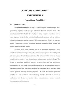
3 Theory Sinusoidal Steady-State Analysis As stated previously, the steady-state behavior of CIRCUITS that are energized by sin- usoidal sources is an important area of study. A sinusoidal voltage source produces a voltage that varies sinusoidally with time. Using the cosine function, we can write a sinusoidally varying voltage as follows v(t) = Vm cos ( t + ) ( ) and the corresponding sinusoidally varying current as i(t) = Im cos ( t + ). ( ) 3 - 2 The plot of sinusoidal voltage versus time is shown in Figure below. Our first observation is that a sinusoidal function is periodic. A periodic function is defined such that y (t) = y (t + T) where T is called the period of the function and is the length of time it takes the sinusoidal function to pass through all of its possible values.

4 The reciprocal of T gives the number of cycles per second, or frequency, of the sine wave and is denoted by f; thus f = 1/T. ( ) A cycle per second is referred to as a Hertz and is abbreviated Hz. Omega, ( ), is used to represent the angular or radian frequency of the sinusoidal function; thus = 2 f = 2 / T radians/second. ( ) 3 - 3 Figure : A Sinusoidal Voltage Equation ( ) is derived from the fact that the cosine function passes through a complete set of values each time its argument passes through 2 radians (360o). From Equation ( ), we see that whenever t is an integral multiple of T, the argument t increases by an integral multiple of 2 radians. The maximum amplitude of the sinusoidal voltage shown in Figure is given by the coefficient Vm and is called the peak voltage.

5 It follows that the peak-to-peak voltage is equal to 2Vm. The phase angle of the sinusoidal voltage is the angle . It determines the value of the sinusoidal function at t = 0. Changing the value of the phase angle shifts the sinusoidal function along the time axis, but has no effect on either the amplitude (Vm) or the angular frequency ( ). Note that is normally given in degrees. It follows that t must be converted from radians to degrees before the two quantities can be added. In summary, a major point to recognize is that a sinusoidal function can be completely specified by giving its maximum amplitude (either peak or peak-to-peak value), frequency, and phase angle. In general, there are three important criteria to remember regarding the steady-state response of a linear network ( , CIRCUITS consisting of resistors, inductors, and capacitors) excited by a sinusoidal source.

6 (1) The steady-state response is a sinusoidal function. (2) The frequency of the response signal is identical to the frequency of the source signal. (3) The amplitude and phase angle of the response will most likely differ from the amplitude and phase angle of the source and are dependent on the values of the resistors, inductors, and capacitors in the Circuit as well as the frequency of the source signal. 3-4 jmeVV= sincosmmjVVV+=It follows then the problem of finding the steady-state response is reduced to finding the maximum amplitude and phase angle of the response signal since the waveform and frequency of the response are the same as the source signal. In analyzing the steady-state response of a linear network, we use the phasor, which is a complex number that carries the amplitude and phase angle information of a sinusoidal function.

7 Given the sinusoidal voltage defined previously in Equation ( ), we define the phasor representation as ( ) where V, is the maximum amplitude , the peak voltage and is the phase angle of the sinusoidal function. Equation ( ) is the polar form of a phasor. A phasor can also be expressed in rectangular form. Thus, Equation ( ) can be written as ( ) In an analogous manner, the phasor representation of the sinusoidal current defined in Equation ( ) is defined as I = Im ej = Im cos + jIm sin . ( ) We will find both the polar form and rectangular form useful in Circuit applications of the phasor concept.

8 Also, the frequent occurrence of the exponential function ej has led to a shorthand notation called the angle notation such that Vm / Vm e j ( ) and Im / Im e j ( ) 3-5 Thus far, we have shown how to move from a sinusoidal function ( , the time domain) to its phasor transform ( , the complex domain). It should be apparent that we can reverse the process. Thus, given the phasor, we can write the expression for the sinusoidal function. As an example, if we are given the phasor V = 5/36o , the expression for v(t) in the time domain is v(t) = 5 cos( t + 36o), since we are using the cosine function for our sinusoidal reference function. Now, the systematic application of the phasor transform in Circuit Analysis re- quires that we introduce the concept of impedance.

9 In general, we find that the voltage-current relationship of a linear Circuit element is given by V = Z I ( ) where Z is the impedance of the Circuit element. The impedance of each of the three linear Circuit elements is given as follows: (a) The impedance (ZR) of a resistor is R in rectangular form and R / 0o in angle form. From Equation ( ), we see that the phasor voltage at the terminals of a resistor equals R times the phasor current. The phasor-domain equivalent Circuit for the resistor Circuit is shown in Figure (a). If it is assumed that the current through the resistor is given by the phasor I = Im / , then the voltage across the resistor is V = R I = (R / 0o )(Im / ) = R Im / ( ) from which we observe that there is no phase shift between the current and voltage.

10 3 - 6 Figure Phasor Domain Equivalent CIRCUITS (b) The impedance (ZL) of an inductor is j L in rectangular form and L/ 90o in angle form. Again, from Equation ( ), we see that the phasor voltage at the terminals of an inductor equals j L times the phasor current. The phasor-domain equivalent Circuit for the inductor is shown in Figure (b). If we assume I = Im / , then the voltage is given by V = (j L) I = ( L / 90o )(Im / ) = LIm / + 90o ( ) from which we observe that the voltage and current will be out of phase by exactly 90o. In particular, the voltage will lead the current by 90o or, what is equivalent, the current will lag behind the voltage by 90o. (c) The impedance (ZC) of a capacitor is l/j C (or -j/ C) in rectangular form and 1/ C/ -90o in angle form.