Transcription of Computer Graphics Lecture Notes - Dynamic Graphics Project
1 Computer Graphics Lecture NotesCSC418 / CSCD18 / CSC2504 Computer Science DepartmentUniversity of TorontoVersion: November 24, 2006 Copyrightc 2005 David Fleet and Aaron HertzmannCSC418 / CSCD18 / CSC2504 CONTENTSC ontentsConventions and Notationv1 Introduction to Displays .. Line Drawing .. Curves .. and Normals .. Curves in OpenGL .. Transformations .. Transformations .. Coordinates .. and Abuses of Homogeneous Coordinates .. Transformations .. in OpenGL .. 164 Coordinate Free Geometry1853D Representations .. Tangents and Normals .. on Surfaces .. Form .. Form .. Surfaces .. Patch .. of Revolution .. Mesh .. Affine Transformations .. Coordinates .. of a Point About a Line.
2 Transformations .. 30 Copyrightc 2005 David Fleet and Aaron HertzmanniCSC418 / CSCD18 / Triangle Meshes .. Triangle Meshes .. 316 Camera Lens Model .. Camera Model .. Projections .. Projection .. Position and Orientation .. Projection .. Perspective .. a Triangle .. Camera Projections in OpenGL .. View Volume and Clipping .. Removal .. Depth Buffer .. s Algorithm .. Trees .. in OpenGL .. 498 Basic Lighting and Reflection Models .. Reflection .. Specular Reflection .. Specular Reflection .. Illumination .. Reflectance Model .. in OpenGL .. Shading .. Shading .. in OpenGL .. 5810 Texture Overview .. Texture Sources.
3 Texture Procedures .. Digital Images ..60 Copyrightc 2005 David Fleet and Aaron HertzmanniiCSC418 / CSCD18 / Mapping from Surfaces into Texture Space .. Textures and Phong Reflectance .. Aliasing .. Texturing in OpenGL .. 6211 Basic Ray Basics .. Ray Casting .. Intersections .. Triangles .. General Planar Polygons .. Spheres .. Affinely Deformed Objects .. Cylinders and Cones .. The Scene Signature .. Efficiency .. Surface Normals at Intersection Points .. Affinely-deformed surfaces.. Shading .. Basic (Whitted) Ray Tracing .. Texture .. Transmission/Refraction .. Shadows .. 7312 Radiometry and Geometry of lighting.
4 Elements of Radiometry .. Basic Radiometric Quantities .. Radiance .. Bidirectional Reflectance Distribution Function .. Computing Surface Radiance .. Idealized Lighting and Reflectance Models .. Diffuse Reflection .. Ambient Illumination .. Specular Reflection .. Phong Reflectance Model ..9113 Distribution Ray Problem statement .. Numerical integration .. Simple Monte Carlo integration .. 94 Copyrightc 2005 David Fleet and Aaron HertzmanniiiCSC418 / CSCD18 / Integration at a pixel .. Shading integration .. Stratified Sampling .. Non-uniformly spaced points .. Importance sampling .. Distribution Ray Tracer .. 9814 Interpolation Basics.
5 Catmull-Rom Splines .. 10115 Parametric Curves And Parametric Curves .. B ezier curves .. Control Point Coefficients .. B ezier Curve Properties .. Rendering Parametric Curves .. B ezier Surfaces .. 10916 Overview .. Keyframing .. Kinematics .. Forward Kinematics .. Inverse Kinematics .. Motion Capture .. Physically-Based Animation .. Single 1D Spring-Mass System .. 3D Spring-Mass Systems .. Simulation and Discretization .. Particle Systems .. Behavioral Animation .. Data-Driven Animation .. 120 Copyrightc 2005 David Fleet and Aaron HertzmannivCSC418 / CSCD18 / CSC2504 AcknowledgementsConventions and NotationVectors have an arrow over their variable name:~v.
6 Points are denoted with a bar instead: are represented by an uppercase written with parentheses and commas separating elements, consider a vector to be a columnvector. That is,(x, y) = xy . Row vectors are denoted with square braces and no commas: x y = (x, y)T= xy set of real numbers is represented byR. The real Euclidean plane isR2, and similarly Eu-clidean three-dimensional space isR3. The set of natural numbers (non-negative integers) is rep-resented are some notable differences between the conventionsused in these Notes and those foundin the course text. Here, coordinates of a point pare written aspx,py, and so on, where the bookuses the notationxp,yp, etc. The same is true for :Text in aside boxes provide extra background or information that you are not re-quired to know for this to Tina Nicholl for feedback on these Notes .
7 Alex Kolliopoulos assisted with electronicpreparation of the Notes , with additional help from 2005 David Fleet and Aaron HertzmannvCSC418 / CSCD18 / CSC2504 Introduction to Graphics1 Introduction to Raster DisplaysThe screen is represented by a 2D array of locations in on an image made up of pixelsThe convention in these Notes will follow that of OpenGL, placing the origin in the lower leftcorner, with that pixel being at location(0,0). Be aware that placing the origin in the upper left isanother common of2 Nintensities or colors are associated with each pixel, whereNis the number of bits perpixel. Greyscale typically has one byte per pixel, for28= 256intensities. Color often requiresone byte per channel, with three color channels per pixel: red, green, and data is stored in aframe buffer.
8 This is sometimes called an image map or operations: setpixel(x, y, color)Sets the pixel at position(x, y)to the given color. getpixel(x, y)Gets the color at the pixel at position(x, y).Scan conversionis the process of converting basic, low level objects into their correspondingpixel map representations. This is often an approximation to the object, since the frame buffer is adiscrete 2005 David Fleet and Aaron Hertzmann1 CSC418 / CSCD18 / CSC2504 Introduction to GraphicsScan conversion of a Basic Line DrawingSet the color of pixels to approximate the appearance of a line from(x0, y0)to(x1, y1).It should be straight and pass through the end points. independent of point order. uniformly bright, independent of explicit equation for a line isy=mx+ :Given two points(x0, y0)and(x1, y1)that lie on a line, we can solve formandbforthe line.
9 Considery0=mx0+bandy1=mx1+ solve form=y1 y0x1 x0andb=y0 in the value forb, this equation can be written asy=m(x x0) + this simple line drawing algorithm:int xfloat m, ym = (y1 - y0) / (x1 - x0)for (x = x0; x <= x1; ++x) {y = m*(x - x0) + y0setpixel(x, round(y), linecolor)}Copyrightc 2005 David Fleet and Aaron Hertzmann2 CSC418 / CSCD18 / CSC2504 Introduction to GraphicsProblems with this algorithm: Ifx1< x0nothing is :Switch the order of the points ifx1< x0. Consider the cases whenm <1andm >1:(a)m <1(b)m >1A different number of pixels are on, which implies differentbrightness between the :Whenm >1, loop overy=y0.. y1instead ofx, thenx=1m(y y0) +x0. Inefficient because of the number of operations and the use offloating point :A more advanced algorithm, called Bresenham s Line Drawing 2005 David Fleet and Aaron Hertzmann3 CSC418 / CSCD18 / CSC2504 Curves2 Parametric CurvesThere are multiple ways to represent curves in two dimensions: Explicit:y=f(x), givenx, :The explicit form of a line isy=mx+b.
10 There is a problem with thisrepresentation what about vertical lines? Implicit:f(x, y) = 0, or in vector form,f( p) = :The implicit equation of a line through p0and p1is(x x0)(y1 y0) (y y0)(x1 x0) = : The direction of the line is the vector~d= p1 p0. So a vector from p0to any point on the line must be parallel to~d. Equivalently, any point on the line must have direction from p0perpendic-ular to~d = (dy, dx) ~ can be checked with~d ~d = (dx, dy) (dy, dx) = 0. So for any point pon the line,( p p0) ~n= ~n= (y1 y0, x0 x1). This is called anormal. Finally,( p p0) ~n= (x x0, y y0) (y1 y0, x0 x1) = , theline can also be written as:( p p0) ~n= 0 Example:The implicit equation for a circle of radiusrand center pc= (xc, yc)is(x xc)2+ (y yc)2=r2,or in vector form,k p pck2= 2005 David Fleet and Aaron Hertzmann4 CSC418 / CSCD18 / CSC2504 Curves Parametric: p= f( )where f:R R2, may be written as p( )or(x( ), y( )).