Transcription of CS231A Course Notes 3: Epipolar Geometry
1 CS231A Course Notes 3: Epipolar GeometryKenji Hata and Silvio Savarese1 IntroductionPreviously, we have seen how to compute the intrinsic and extrinsic param-eters of a camera using one or more views using a typical camera calibrationprocedure or single view metrology. This process culminated in derivingproperties about the 3D world from one image . However, in general, it is notpossible to recover the entire structure of the 3D world from just one is due to the intrinsic ambiguity of the 3D to the 2D mapping: someinformation is simply 1: A single picture such as this picture of a man holding up theLeaning Tower of Pisa can result in ambiguous scenarios. Multiple views ofthe same scene help us resolve these potential example, in Figure 1, we may be initially fooled to believe that theman is holding up the Leaning Tower of Pisa.
2 Only by careful inspectioncan we tell that this is not the case and merely an illusion based on theprojection of different depths onto the image plane. However, if we were ableto view this scene from a completely different angle, this illusion immediatelydisappears and we would instantly figure out the correct scene focus of these lecture Notes is to show how having knowledge of geom-etry when multiple cameras are present can be extremely helpful. Specifically,we will first focus on defining the Geometry involved in two viewpoints andthen present how this Geometry can aid in further understanding the worldaround Epipolar GeometryFigure 2: The general setup of Epipolar Geometry . The gray region is theepipolar plane. The orange line is the baseline, while the two blue lines arethe Epipolar in multiple view Geometry , there are interesting relationships be-tween the multiple cameras, a 3D point, and that point s projections in eachof the camera s image plane.
3 The Geometry that relates the cameras, pointsin 3D, and the corresponding observations is referred to as theepipolargeometryof a stereo illustrated in Figure 2, the standard Epipolar Geometry setup involvestwo cameras observing the same 3D pointP, whose projection in each ofthe image planes is located atpandp respectively. The camera centersare located atO1andO2, and the line between them is referred to as thebaseline. We call the plane defined by the two camera centers andPtheepipolar plane. The locations of where the baseline intersects the two image2 Figure 3: An example of Epipolar lines and their corresponding points drawnon an image are known as the theepipoleseande . Finally, the lines defined bythe intersection of the Epipolar plane and the two image planes are known astheepipolar lines. The Epipolar lines have the property that they intersectthe baseline at the respective epipoles in the image 4: When the two image planes are parallel, then the epipoleseande are located at infinity.
4 Notice that the Epipolar lines are parallel to theuaxis of each image interesting case of Epipolar Geometry is shown in Figure 4, whichoccurs when the image planes are parallel to each other. When the imageplanes are parallel to each other, then the epipoleseande will be located atinfinity since the baseline joining the centersO1,O2is parallel to the imageplanes. Another important byproduct of this case is that the Epipolar linesare parallel to an axis of each image plane. This case is especially useful3and will be covered in greater detail in the subsequent section on real world situations, however, we are not given the exact location ofthe 3D locationP, but can determine its projection in one of the image planesp. We also should be able to know the cameras locations, orientations, andcamera matrices. What can we do with this knowledge?
5 With the knowledgeof camera locationsO1,O2and the image pointp, we can define the epipolarplane. With this Epipolar plane, we can then determine the Epipolar definition,P s projection into the second imagep must be located on theepipolar line of the second image . Thus, a basic understanding of epipolargeometry allows us to create a strong constraint between image pairs withoutknowing the 3D structure of the 5: The setup for determining the essential and fundamental matrices,which help map points and Epipolar lines across will now try to develop seamless ways to map points and Epipolar linesacross views. If we take the setup given in the original Epipolar geometryframework (Figure 5), then we shall further defineMandM to be the cameraprojection matrices that map 3D points into their respective 2D image planelocations. Let us assume that the world reference system is associated to thefirst camera with the second camera offset first by a rotationRand then bya translationT.
6 This specifies the camera projection matrices to be:M=K[I0]M =K [RT RTT](1)1 This means that Epipolar lines can be determined by just knowing the camera centersO1, O2and a point in one of the imagesp43 The Essential MatrixIn the simplest case, let us assume that we havecanonical cameras, inwhichK=K =I. This reduces Equation 1 toM=[I0]M =[RT RTT](2)Furthermore, this means that the location ofp in the first camera s ref-erence system isRp +T. Since the vectorsRp +TandTlie in the epipolarplane, then if we take the cross product ofT (Rp +T) =T (Rp ), we willget a vector normal to the Epipolar plane. This also means thatp, which liesin the Epipolar plane is normal toT (Rp ), giving us the constraint thattheir dot product is zero:pT [T (Rp )] = 0(3)From linear algebra, we can introduce a different and compact expressionfor the cross product: we can represent the cross product between any twovectorsaandbas a matrix-vector multiplication:a b= 0 azayaz0 ax ayax0 bxbybz = [a ]b(4)Combining this expression with Equation 3, we can convert the crossproduct term into matrix multiplication, givingpT [T ](Rp ) = 0pT[T ]Rp = 0(5)The matrixE= [T ]Ris known as theEssential Matrix, creating a com-pact expression for the Epipolar constraint:pTEp = 0(6)The Essential matrix is a 3 3 matrix that contains 5 degrees of freedom.
7 Ithas rank 2 and is Essential matrix is useful for computing the Epipolar lines associatedwithpandp . For instance,` =ETpgives the Epipolar line in the imageplane of camera 2. Similarly`=Ep gives the Epipolar line in the image planeof camera 1. Other interesting properties of the essential matrix is that itsdot product with the epipoles equate to zero:ETe=Ee = 0. Becausefor any pointx(other thane) in the image of camera 1, the correspondingepipolar line in the image of camera 2,l =ETx, contains the epipolee .Thuse satisfiese T(ETx) = (e TET)x= 0 for all thex, soEe = 0. SimilarlyETe= The Fundamental MatrixAlthough we derived a relationship betweenpandp when we have canoni-cal cameras, we should be able to find a more general expression when thecameras are no longer canonical. Recall that gives us the projection matrices:M=K[I0]M =K [RT RTT](7)First, we must definepc=K 1pandp c=K 1p to be the projections ofPto the corresponding camera images if the cameras were canonical.
8 Recallthat in the canonical case:pTc[T ]Rp c= 0(8)By substituting in the values ofpcandp c, we getpTK T[T ]RK 1p = 0(9)The matrixF=K T[T ]RK 1is known as theFundamental Matrix,which acts similar to the Essential matrix from the previous section butalso encodes information about the camera matricesK,K and the relativetranslationTand rotationRbetween the cameras. Therefore, it is alsouseful in computing the Epipolar lines associated withpandp , even when thecamera matricesK,K and the transformationR,Tare unknown. Similar tothe Essential matrix, we can compute the Epipolar lines` =FTpand`=Fp from just the Fundamental matrix and the corresponding points. One maindifference between the Fundamental matrix and the Essential matrix is thatthe Fundamental matrix contains 7 degrees of freedom, compared to theEssential matrix s 5 degrees of how is the Fundamental matrix useful?
9 Like the Essential matrix, ifwe know the Fundamental matrix, then simply knowing a point in an imagegives us an easy constraint (the Epipolar line) of the corresponding point inthe other image . Therefore, without knowing the actual position ofPin 3 Dspace, or any of the extrinsic or intrinsic characteristics of the cameras, wecan establish a relationship between anypandp . The Eight-Point AlgorithmStill, the assumption that we can have the Fundamental matrix, which isdefined by a matrix product of the camera parameters, seems rather , it is possible to estimate the Fundamental matrix given two imagesof the same scene and without knowing the extrinsic or intrinsic parameters ofthe camera. The method we discuss for doing so is known as theEight-Point6 Figure 6: Corresponding points are drawn in the same color on each of therespective , which was proposed by Longuet-Higgins in 1981 and extendedby Hartley in 1995.
10 As the title suggests, the Eight-Point Algorithm assumesthat a set of at least 8 pairs of corresponding points between two images correspondencepi= (ui,vi,1) andp i= (u i,v i,1) gives us the epipo-lar constraintpTiFp i= 0. We can reformulate the constraint as follows:[uiu iv iuiuiu iviviv iviu iv i1] F11F12F13F21F22F23F31F32F33 = 0(10)Since this constraint is a scalar equation, it only constrains one degree offreedom. Since we can only know the Fundamental matrix up to scale, werequire eight of these constraints to determine the Fundamental matrix:7 u1u 1v 1u1u 1u 1v1v1v 1v1u 1v 11u2u 2v 2u2u 2u 2v2v2v 2v2u 2v 21u3u 3v 3u3u 3u 3v3v3v 3v3u 3v 31u4u 4v 4u4u 4u 4v4v4v 4v4u 4v 41u5u 5v 5u5u 5u 5v5v5v 5v5u 5v 51u6u 6v 6u6u 6u 6v6v6v 6v6u 6v 61u7u 7v 7u7u 7u 7v7v7v 7v7u 7v 71u8u 8v 8u8u 8u 8v8v8v 8v8u 8v 81 F11F12F13F21F22F23F31F32F33 = 0(11)This can be compactly written asWf= 0(12)whereWis anN 9 matrix derived fromN 8 correspondences andfisthe values of the Fundamental matrix we practice, it often is better to use more than eight correspondences andcreate a largerWmatrix because it reduces the effects of noisy solution to this system of homogeneous equations can be found in theleast-squares sense by Singular Value Decomposition (SVD), asWis rank-deficient.