Transcription of Convolution Table (1) Convolution Table (2)
1 Lecture 5 Slide 1 PYKC 24-Jan-11 Signals & Linear Systems Lecture 5 Time-domain analysis: Convolution (Lathi ) Peter Cheung Department of Electrical & Electronic Engineering Imperial College London URL: E-mail: Lecture 5 Slide 2 PYKC 24-Jan-11 Signals & Linear Systems Convolution Integral: System output ( zero-state response) is found by convolving input x(t) with System s impulse response h(t). Convolution Integral ()()*()()()ytxthtxhtd == LTI System Impulse Response h(t) ()()*()ytxtht=Lecture 5 Slide 3 PYKC 24-Jan-11 Signals & Linear Systems Use Table to find Convolution results easily: Convolution Table (1) p177 Lecture 5 Slide 4 PYKC 24-Jan-11 Signals & Linear Systems Convolution Table (2) Lecture 5 Slide 5 PYKC 24-Jan-11 Signals & Linear Systems Convolution Table (3) p177 Lecture 5 Slide 6 PYKC 24-Jan-11 Signals & Linear Systems Example (1) Find the loop current y(t) of the RLC circuits for input when all the initial conditions are zero.
2 We have seen in slide that the system equation is: The impulse response h(t) was obtained in : The input is: Therefore the response is: p178 Lecture 5 Slide 7 PYKC 24-Jan-11 Signals & Linear Systems Example (2) Using distributive property of Convolution : Use Convolution Table pair #4: p178 Lecture 5 Slide 8 PYKC 24-Jan-11 Signals & Linear Systems When input is complex What happens if input x(t) is not real, but is complex? If x(t) = xr(t) + jxi(t), where xr(t) and xi(t) are the real and imaginary part of x(t), then That is, we can consider the Convolution on the real and imaginary components separately. p179 Lecture 5 Slide 9 PYKC 24-Jan-11 Signals & Linear Systems Intuitive explanation of Convolution Assume the impulse response decays linearly from t=0 to zero at t=1.
3 Divide input x( ) into pulses. The system response at t is then determined by x( ) weighted by h(t- ) ( x( ) h(t- )) for the shaded pulse, PLUS the contribution from all the previous pulses of x( ). The summation of all these weighted inputs is the Convolution integral. p191 ()()*()ytxtht=Lecture 5 Slide 10 PYKC 24-Jan-11 Signals & Linear Systems Convolution using graphical method (1) Determine graphically y(t) = x(t)*h(t) for x(t) = e-tu(t) and h(t) = e-2tu(t). p183 Remember: variable of integration is , not t Lecture 5 Slide 11 PYKC 24-Jan-11 Signals & Linear Systems Convolution using graphical method (2) Lecture 5 Slide 12 PYKC 24-Jan-11 Signals & Linear Systems Interconnected Systems Parallel connected system Cascade systems & Commutative property p192 ()xt12() ()* () ()* ()ythtxthtxt=+()xt12() [ ()* ()]* ()yththtxt=Lecture 5 Slide 13 PYKC 24-Jan-11 Signals & Linear Systems Interconnected Systems Integration: Also true for differentiation: Let Then g(t), the step response is: ( x(t) is an impulse, and h(t) is the impulse response of the system) p193 Lecture 5 Slide 14 PYKC 24-Jan-11 Signals & Linear Systems Total Response Let us put everything together, using our RLC circuit as an example.
4 Let us assume In earlier slides, we have shown that p197 x(t)=10e 3tu(t),y(0)=0, y(0)= 5 Slide 15 PYKC 24-Jan-11 Signals & Linear Systems Natural vs Forced Responses Note that characteristic modes also appears in zero-state response (because it has an impact on h(t)). We can collect the e-t and e-2t terms together, and call these the NATURAL response. The remaining e-3t which is NOT a characteristic mode is the FORCED response. p197 Lecture 5 Slide 16 PYKC 24-Jan-11 Signals & Linear Systems Additional Example *