Transcription of Data Normalization for Dummies Using SAS - …
1 Venu Perla, Philadelphia Area SAS Users Group (PhilaSUG) Winter 2016 Meeting; March 16, 2016 Philadelphia University, Philadelphia, PA, USA 1 data Normalization for Dummies Using SAS Venu Perla, Clinical Programmer, Emmes Corporation, Rockville, MD 20850 SAS Certified Base Programmer for SAS 9 SAS Certified Advanced Programmer for SAS 9 SAS Certified Clinical Trials Programmer Using SAS 9 SAS Certified Statistical Business Analyst Using SAS 9: Regression and Modeling Abstract Life scientists often struggle to normalize non-parametric data or ignore Normalization prior to data analysis. Based on statistical principles, logarithmic, square-root and arcsine transformations are commonly adopted to normalize non-parametric data for parametric tests.
2 Several other transformations are also available for normalizing data . However, for many, identification of right transformation for non-parametric data is a tricky job. The objective of this paper is to develop a SAS program that identifies right transformation and normalize non-parametric data for regression analysis. To achieve this objective, PROC SQL, PROC TRANSREG, PROC REG, PROC UNIVARIATE, PROC STDIZE, PROC CORR, PROC SGPLOT, PROC IMPORT and PROC PRINT of SAS are utilized in this paper. Finally, SAS MACROS are developed on this code for reuse without hassles. 1. Introduction Figure 1 Are you a dummy? Are you lazy? Do you really have no time? If your answer is Yes to any of these questions, and if you are performing regression analysis, read this paper and apply steps mentioned here to normalize your data Using SAS.
3 If your answer is No to all the questions, and if you are performing regression analysis, then you may have to apply formal statistical knowledge to normalize your data (Figure 1). Formal statistics include several transformations (logarithmic, square-root, arcsine etc) that are based on certain rules. However, SAS programming steps mentioned in in this paper are not intended to replace formal statistical knowledge existing elsewhere. In other words, this paper is intended for true or conditional Dummies . Parametric tests, such as an ANOVA, t-test or linear regression, can be applied to a dataset if it meets certain assumptions. One of the assumptions is that the data should be normally distributed. Parametric tests on non-normal data produce false results. The objective of this paper is to show how 6-step protocol transforms a dataset from non-parametric to parametric for regression analysis.
4 It is important to note that the variables used in the parametric analysis must be continuous in nature (quantitative, interval or ratio values). Discrete variables (categorical, qualitative, nominal or ordinal values) are not right candidates for parametric analysis. A raw data on two interrelated plant metabolites (X and Y) is tested and normalized in this paper. There are 51 observations in this replicated data . data analysis is carried out by SAS software with windows operating Venu Perla, Philadelphia Area SAS Users Group (PhilaSUG) Winter 2016 Meeting; March 16, 2016 Philadelphia University, Philadelphia, PA, USA 2 system. data used in this paper is imported from a sheet (XY_Data) of Microsoft Office Excel 97-2003 file ( ) (see XY_Data in Appendix).
5 PROC IMPORT is utilized to import XY_Data and renamed it as HEALTH (Table 1). %let path= C:\Users\Perla\Desktop\; title "Importing data from excel"; proc import file="& " out=health replace dbms=xls; sheet=XY_Data; getnames=yes; run; title "Checking imported data "; proc print data =health; run; For importing XY_Data, macro EXCEL_IMPORT is developed on above code (see Appendix). This macro can be utilized in future for analysis of similar data by running following code: %excel_import (excel_file= , excel_sheet= , dataset=); 2. data Normalization After importing data into SAS, a 6-step protocol for Normalization of data for regression analysis Using SAS is presented in Figure 2. Programming aspects of each step are also discussed in this section. Step 1: Check Scatter Plot and Correlation Matrix Relationship between X- and Y-variables can be visualized Using PROC SGPLOT and PROC CORR.
6 Ods graphics on; title "Scatter plot of X and Y"; proc sgplot data = health; scatter x=x y=y; run; title "Correlation between X and Y"; proc corr data = health; var x y; run; ods graphics off; Scatter plot of X and Y indicates that there is no clear relationship between these two variables (Figure 3). Results on Pearson correlation coefficients indicate a weak correlation between X- and Y-variables (Table 2). Venu Perla, Philadelphia Area SAS Users Group (PhilaSUG) Winter 2016 Meeting; March 16, 2016 Philadelphia University, Philadelphia, PA, USA 3 Figure 2 Figure 3 Table 2 Above code is utilized to develop a macro, SCATTER_CORR (See Appendix). This macro can be utilized in future for analysis of similar data by running following code: %scatter_corr (dataset= , xvar= , yvar= ); Venu Perla, Philadelphia Area SAS Users Group (PhilaSUG) Winter 2016 Meeting; March 16, 2016 Philadelphia University, Philadelphia, PA, USA 4 Step 2: Perform Regression Analysis and Normality Tests There is an indication of a weak correlation between X and Y (Pearson correlation coefficient: ).
7 Further analysis is carried out on this raw data Using PROC REG and PROC UNIVARIATE. LACKFIT option of MODEL statement in PROC REG determines whether this linear model is a good fit for this replicated data or not? Residual analysis and normality tests are carried out Using PROC UNIVARIATE with NORMAL option. If data is normal after 2nd step, no further steps are required to execute to normalize the data . ODS graphics on; title "Regression analysis"; proc reg data = health plots(only)=diagnostics (unpack); model y = x/lackfit; output out =mdlres r=resid; run; ODS graphics off; proc univariate data = mdlres normal; var resid; run; Analysis of variance indicates that LACK OF FIT for the linear model is significant (Table 3). This suggests that further in-depth analysis has to be carried out on this raw data before rejecting the model.
8 Parameter estimates and adjusted R2 value for the raw data are provided in Table 4A and 4B, respectively. Adjusted R2 value is negligible ( ). Distribution of residuals for Y is not normal for the raw data (Figure 4). Venu Perla, Philadelphia Area SAS Users Group (PhilaSUG) Winter 2016 Meeting; March 16, 2016 Philadelphia University, Philadelphia, PA, USA 5 Figure 4 Furthermore, significant p values for four tests of normality are the true testimony of non-normal distribution of data (Table 5). Table 5 Above code is utilized to develop a macro REG_NORMALITY (See Appendix). This macro can be utilized in future for analysis of similar data by running following code: %reg_normality (dataset=health, xvar=x, yvar=y); Step 3: Transform data into Non-zero and Non-negative data Box-Cox power transformation can be adopted to normalize this raw data .
9 data should be converted to non-zero and non-negative values before testing for Box-Cox power transformation. Following code transforms X- and Y-variables into non-zero and/or non- negative variables only when 0 or negative values are encountered in the data . PROC SQL is used to transform X- and Y-variable data into non-zero and non-negative data . Table HEALTH_COX is created from dataset HEALTH in this procedure. Proc SQL reproduced original data as there are no zeros and no negative values (Table 6). title "Transforming X and Y values into non-zero and non-negative values"; proc sql; create table health_cox as select case when min(x) <=0 then (-(min(x))+x+1) else x end as X, case when min(y) <=0 then (-(min(y))+y+1) else y end as Y from health; quit; proc print data =health_cox; Venu Perla, Philadelphia Area SAS Users Group (PhilaSUG) Winter 2016 Meeting; March 16, 2016 Philadelphia University, Philadelphia, PA, USA 6 run; Table 6 Macro TRANSFORM_ZERO_NEG is developed for above PROC SQL code (See Appendix).
10 This macro can be invoked in future by following statement: %transform_zero_neg (dataset= ,xvar= ,yvar= ,pre_trans_dataset= ); Step 4: Perform Box-Cox Power Transformation Box-Cox power transformation on non-zero and non-negative data is performed Using PROC TRANSREG with ODS GRAPHICS on. title "Box-Cox power transformation: Identification of right exponent (Lambda)"; ods graphics on; proc transreg data = health_cox; model boxcox(y) = identity(x); run; ods graphics off; Above code generated Box-Cox analysis for Y (Figure 5). Selected lambda ( at 95% CI) is the exponent to be used to transform the data into normal shape. Figure 5 In order to get convenient lambda value, above SAS code is executed without ODS GRAPHICS statement. proc transreg data = health_cox; model boxcox(y)=identity(x); run; Venu Perla, Philadelphia Area SAS Users Group (PhilaSUG) Winter 2016 Meeting; March 16, 2016 Philadelphia University, Philadelphia, PA, USA 7 This code generated best lambda, lambda with 95% confidence interval, and convenient lambda (Table 7).