Transcription of 158-2009: Using PROC SGPLOT for Quick High …
1 Paper 158-2009 1 Using PROC SGPLOT for Quick high -Quality Graphs Lora D. Delwiche, University of California, Davis, CA Susan J. Slaughter, Avocet Solutions, Davis, CA ABSTRACT New with SAS , ODS Graphics introduces a whole new way of generating high quality graphs Using SAS. With just a few lines of code, you can add sophisticated graphs to the output of existing statistical procedures, or create stand-alone graphs. The SGPLOT procedure produces a variety of graphs including bar charts, scatter plots, and line graphs. Because ODS Graphics uses the Output Delivery System, graphs can be sent to ODS destinations, and use ODS styles. This paper shows how to produce different types of graphs Using PROC SGPLOT , how to send your graph to different ODS destinations, and how to apply ODS styles to your graph. We will also show how to use the ODS Graphics Editor to make changes to graphs produced Using ODS Graphics.
2 INTRODUCTION When ODS Graphics was originally conceived, the goal was to enable statistical procedures to produce sophisticated graphs tailored to each specific statistical analysis, and to integrate those graphs with the destinations and styles of the Output Delivery System. In SAS , over 60 statistical procedures have the ability to produce graphs Using ODS Graphics. A fortuitous side effect of all this graphical power has been the creation of a set of procedures for creating stand-alone graphs (graphs that are not embedded in the output of a statistical procedure). These procedures all have names that start with the letters SG ( SGPLOT , SGSCATTER, SGPANEL, and SGRENDER). This paper focuses on one of those new procedures, the SGPLOT procedure. PROC SGPLOT produces many types of graphs. In fact, this one procedure produces 15 types of graphs. PROC SGPLOT creates one or more graphs and overlays them on a single set of axes.
3 (There are four axes in a set: left, right, top, and bottom.) Other SG procedures create panels with multiple sets of axes, or render graphs Using custom ODS graph templates. Because the syntax for SGPLOT and SGPANEL are so similar, we also show an example of SGPANEL which produces a panel of graphs all Using the same axis specifications. ODS GRAPHICS VS. TRADITIONAL SAS/GRAPH To use ODS Graphics you must have SAS/GRAPH software which is licensed separately from Base SAS. Some people may wonder whether ODS Graphics replaces traditional SAS/Graph procedures. No doubt, for some people and some applications, it will. But ODS Graphics is not designed to do everything that traditional SAS/Graph does, and does not replace it. For example, ODS Graphics does not create contour plots; for contour plots you need to use traditional SAS/GRAPH. Here are some of the major differences between ODS Graphics and traditional SAS/GRAPH procedures.
4 Traditional SAS/GRAPH ODS Graphics Graphs are saved in SAS graphics catalogs Produces graphs in standard image file formats such as PNG and JPEG Graphs are viewed in the Graph window Graphs are viewed in standard viewers such as a web browser for HTML output Uses GOPTIONS statements to control appearance of graphs Uses ODS styles to control appearance of graphs. Hands-on WorkshopsSASG lobalForum2009 2 VIEWING ODS GRAPHICS When you produce ODS Graphics in the SAS windowing environment, for most destinations the Results Viewer window opens displaying your results. However, when you use the LISTING destination, graphs are not automatically displayed. You can always view your graphs by double-clicking their graph icons in the Results window. EXAMPLES HISTOGRAMS Histograms show the distribution of a continuous variable. The following PROC SGPLOT uses data from the preliminary heats of the 2008 Olympics Men s Swimming Freestyle 100 m event.
5 The histogram shows a variable, TIME, which is the time in seconds for each swimmer. * Histograms; PROC SGPLOT DATA = Freestyle; HISTOGRAM Time; TITLE "Olympic Men's Swimming Freestyle 100"; RUN; Hands-on WorkshopsSASG lobalForum2009 3 The next PROC SGPLOT uses a HISTOGRAM statement with a DENSITY statement to overlay a density plot on top of the histogram. The default density plot is the normal distribution. When overlaying plots, the order of the statements determines which plot is on top. The plot resulting from the first statement will be on the bottom, followed by any subsequent plots. PROC SGPLOT DATA = Freestyle; HISTOGRAM Time; DENSITY Time; TITLE "Olympic Men's Swimming Freestyle 100"; RUN; BAR CHARTS Bar charts show the distribution of the values of a categorical variable. This code uses a VBAR statement with the variable REGION.
6 The chart shows the number of countries in each region that participated in the 2008 Olympics. * Bar Charts; PROC SGPLOT DATA = Countries; VBAR Region; TITLE 'Olympic Countries by Region'; RUN; Hands-on WorkshopsSASG lobalForum2009 4 This bar chart is like the first one except that the bars have been divided into groups Using the GROUP= option. The grouping variable is a categorical variable named POPGROUP. The GROUP= option can be used with many SGPLOT statements (see Table 1). PROC SGPLOT DATA = Countries; VBAR Region / GROUP = PopGroup; TITLE 'Olympic Countries by Region and Population Group'; RUN; In this code, a RESPONSE= option has been added. The response variable is NUMPARTICIPANTS, the number of participants in the 2008 Olympics from each country. Now each bar represents the total number of participants for a region. PROC SGPLOT DATA = Countries; VBAR Region / RESPONSE = NumParticipants; TITLE 'Olympic Participants by Region'; RUN; Hands-on WorkshopsSASG lobalForum2009 5 SERIES PLOTS In a series plot, the data points are connected by a line.
7 This example uses the average monthly rainfall for three cities, Beijing, Vancouver and London. Three SERIES statements overlay the three lines. Data for series plots must be sorted by the X variable. If your data are not already in the correct order, then use PROC SORT to sort the data before running the SGPLOT procedure. * Series plot; PROC SGPLOT DATA = Weather; SERIES X = Month Y = BRain; SERIES X = Month Y = VRain; SERIES X = Month Y = LRain; TITLE 'Average Monthly Rainfall in Olympic Cities'; RUN; EMBELLISHING GRAPHS So far the examples have all shown how to create basic plots. The remaining examples show statements and options you can use to polish graphs. XAXIS AND YAXIS STATEMENTS In the preceding series plot, the variable on the X axis is Month. The values of Month are integers from 1 to 12, but the default labels on the X axis have values like The option TYPE = DISCRETE tells SAS to use the actual data values.
8 Other options change the axis label and set values for the Y axis, and add grid lines. * Plot with XAXIS and YAXIS; PROC SGPLOT DATA = Weather; SERIES X = Month Y = BRain; SERIES X = Month Y = VRain; SERIES X = Month Y = LRain; XAXIS TYPE = DISCRETE GRID; YAXIS LABEL = 'Rain in Inches' GRID VALUES = (0 TO 10 BY 1); TITLE 'Average Monthly Rainfall in Olympic Cities'; RUN; Hands-on WorkshopsSASG lobalForum2009 6 PLOT STATEMENT OPTIONS Many options can be added to plot statements. For these SERIES statements, the options LEGENDLABEL=, MARKERS, AND LINEATTRS= have been added. The LEGENDLABEL= option can be used with any of the plot statements, while the MARKERS and LINEATTRS= options can only be used with some plot statements (see Table 1). * Plot with options on plot statements; PROC SGPLOT DATA = Weather; SERIES X = Month Y = BRain / LEGENDLABEL = 'Beijing' MARKERS LINEATTRS = (THICKNESS = 2); SERIES X = Month Y = VRain / LEGENDLABEL = 'Vancouver' MARKERS LINEATTRS = (THICKNESS = 2); SERIES X = Month Y = LRain / LEGENDLABEL = 'London' MARKERS LINEATTRS = (THICKNESS = 2); XAXIS TYPE = DISCRETE; TITLE 'Average Monthly Rainfall in Olympic Cities'; RUN; Hands-on WorkshopsSASG lobalForum2009 7 REFLINE STATEMENT Reference lines can be added to any type of graph.
9 In this case, lines have been added marking the average rainfall per month for the entire year for each city. The TRANSPARENCY= option on the REFLINE statement specifies that the reference line should be 50% transparent. The TRANSPARENCY option can also be used with other plot statements (see Table 1). * Plot with REFLINE; PROC SGPLOT DATA = Weather; SERIES X = Month Y = BRain; SERIES X = Month Y = VRain; SERIES X = Month Y = LRain; XAXIS TYPE = DISCRETE; REFLINE / TRANSPARENCY = LABEL = ('Beijing(Mean)' 'Vancouver(Mean)' 'London(Mean)'); TITLE 'Average Monthly Rainfall in Olympic Cities'; RUN; INSET STATEMENT The INSET statement allows you to add descriptive text to plots. Insets can be added to any type of graph. * Plot with INSET; PROC SGPLOT DATA = Weather; SERIES X = Month Y = BRain; SERIES X = Month Y = VRain; SERIES X = Month Y = LRain; XAXIS TYPE = DISCRETE; INSET 'Source Lonely Planet Guide'/ POSITION = TOPRIGHT BORDER; TITLE 'Average Monthly Rainfall in Olympic Cities'; RUN; Hands-on WorkshopsSASG lobalForum2009 8 SYNTAX The SGPLOT procedure can produce 15 different types of plots that can be grouped into five general areas: basic X Y plots, band plots, fit and confidence plots, distributions graphs for continuous DATA, and distribution graphs for categorical DATA.
10 Many of these plot types can be used together in the same graph. In the examples, we used the HISTOGRAM and DENSITY statements together to produce a histogram overlaid with a normal density curve. We also used three SERIES statements together to produce one graph with three different series lines. However not all plot statements can be used with all other plot statements. Table 1 shows which statements can be used with which other statements. Table 1 also includes several options that can be used with many different plot statements as well as selected optional statements. Hands-on WorkshopsSASG lobalForum2009 9 Table 1. Compatibility of SGPLOT procedure statements and selected options. If a check mark appears in the box then the two statements or options can be used together. SCATTER SERIES STEP NEEDLE BAND REG LOESS PBSPLINE ELLIPSE HBOX/VBOX HISTOGRAM DENSITY HBAR/VBAR HLINE/VLINE DOT Basic X Y PLots PLOTNAME X=var Y=var / options; SCATTER 9 99999999 SERIES 9 99999999 STEP 9 99999999 NEEDLE 9 99999999 Band Plots BAND X=var UPPER=var LOWER=var / options; (You can also specify numeric values for upper and lower.)