Di erential Equations - Theory and Applications - Version ...

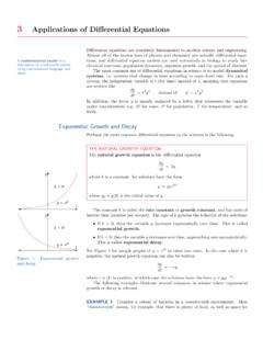
1 Differential Equations - Theory and Applications - Version : Fall 2017 Andr as Domokos , PhDCalifornia State University, SacramentoContentsChapter 0. Introduction3 Chapter 1. Calculus review. Differentiation and integration Antiderivatives and Indefinite Definite Integrals11 Chapter 2. Introduction to Differential Initial value Classifications of Examples of DEs modelling real-life phenomena25 Chapter 3. First order differential Equations solvable by analytical Differential Equations with separable First order linear differential Bernoulli s differential Non-linear homogeneous differential Differential Equations of the formy (t) =f(at+by(t) +c).

2 second order differential Equations reducible to first order differential Equations 42 Chapter 4. General Theory of differential Equations of first Slope fields (or direction fields) first order differential Existence and uniqueness of solutions for initial value The method of successive Numerical methods for Differential The Euler s The improved Euler (or Heun) The fourth order Runge-Kutta NDSolve command in Mathematica71 Chapter 5. Higher order linear differential General Linear and homogeneous DEs with constant Linear and non-homogeneous DEs with constant Variation of parameters for second order linear The undetermined coefficients method and the superposition Use Mathematica to solve higher order The Cauchy-Euler DE88 Chapter 6.

3 Solving linear differential Equations with the Laplace Definition and properties of the Laplace Further properties of the Laplace transform. Transforms of the Heavisidefunction and the Dirac Delta Translation on Derivatives of the Laplace The Laplace transform of the unit step function and of piecewise The Dirac Delta The inverse Laplace Calculate the Laplace transform and inverse Laplace transform Solving IVPs of linear DEs with the Laplace Solving differential Equations using Mathematica and the Laplace transform Solving systems of first order linear differential Equations with the Using Mathematica to solve systems of DEs115 Chapter 7.

4 Appendix: Mathematica files1172 CHAPTER 0 IntroductionThis textbook covers the material for the undergraduate Differential Equations courseat California State University Sacramento. Although there might be issues related just toa particular campus, I believe that the presentation shown here is useful to a general , let s see the particular issues. This is a 3 unit class, taught 3 times 50 minutes(or 2 times 75 minutes) per week during a semester of 15 weeks. Most of the students arescience majors, including mathematics, physics and engineering. Many of the students aretransfer students, who took the prerequisite classes - Precalculus, Calculus 1 and 2 - at othercampuses, so there is a wide range of mathematical knowledge and the beginning of every semester a week of review of calculus, especially differentiationand integration rules, proved to be Linear Algebra course is not a prerequisite for this class, and within the time frameallowed, it is difficult to spend time on covering the complete fundamentals regarding opera-tions with matrices, eigenvalues and eigenvectors.

5 Also, there is no computer lab componentfor this course. These are not optimal starting points for this class and I hope that thecoming years will bring some , let s talk about some general issues. Almost all of my students were used togetting the 1000+ pages textbooks for their earlier courses. Over the years these huge text-books killed the habits of taking time to read them, focus on the details and understandingthe definitions and theorems describing the main ideas. The most frequent question I do getis: We see what is the material, but how much of it we have to know for the exam? Theanswer - All of it. - usually brings out a big sign of Equations is a very important mathematical subject from both theoreticaland practical theoretical importance is given by the fact that most pure mathematics theorieshave Applications in Differential Equations .

6 For students, all the prerequisite knowledge istested in this practical importance is given by the fact that the most important time dependentscientific, social and economical problems are described by differential, partial differentialand stochastic differential Equations . The bridge between Nature or Universe and us is pro-vided by mathematical modeling, which is the process of finding the correct mathematicalequations describing a certain problem. This process might start with experimental mea-surements and analysis, which lead to certain Equations , in our case differential , these differential Equations are solved and their solutions tested for agreement to ex-perimental results.

7 In this process we generate some solutions, which have the role to predict3thefuture behaviorof the analyzed general, regarding the future, there is no solution manual and here comes another of my students were used to having solution manuals for their mathematics classes andchecking whether the solution is right or wrong was reduced to comparison with the answersin the solution manual. However, this eliminates the need to completely understand whatwe are doing and whether the answer really makes Equations is probably one of the best classes which can make us understandthat Nature does not provide us with a complete solution manual. We usually have to findsome approximate answers and we are also left with the task of predicting how accuratethese answers are, without knowing the correct this reason, there will be NO SOLUTION MANUAL posted.

8 I request the studentsto check the correctness of their answers by applying the theoretical methods shown in class,but also by using a computer software in the campus computer labs. The available softwareis Mathematica, which could be substituted off campus by Wolfram Alpha. There are manymathematical softwares, like Maple, Matlab, Octave, and you are free to use whichever isavailable to you. The most important thing is to actively participate in the teaching-learningprocess and based on the information presented in class, create your own way of checkingyour answers. The answers given by computers might be in a different form than the onesobtained on paper, but it is a good challenge to compare them.

9 You must develop intuition,theoretical and computer knowledge to be able to test and decide whether a solution iscorrect or 1 Calculus review. Differentiation and integration a functiony:I R, whereIis an interval on the real lineR. We say that the functionyhas a derivative att0 Iif the limitlimt I,t t0y(t) y(t0)t t0exists and it is finite. In the case when the derivative exists, we use the notationy (t0) = limt I,t t0y(t) y(t0)t notations for the derivative of functionyatt0can bedydt(t0) orddty(t0).In caset0is one of the endpoints of the intervalI, then the above limits become one the derivative exists at everyt0 I, theny (t) is a new function, called the (t) has a derivative function, then we call it the second derivative of the functiony(t)and denote it byy (t).

10 For higher order derivatives we use the notationsy (t),y(4)(t), .. ,y(n)(t), ordndtny(t).Interpretations and Applications of the derivative:(1)y (t0) is the instantaneous rate of change of the functionyatt0.(2)y (t0) is the slope of the tangent line to the curvey=y(t), t Iat the point(t0,y(t0)).(3) If the functionyhas a local maximum (minimum) att0, which is in the interior ofI, andyis differentiable att0, theny (t0) = 0. However,y (t0) might not be zero ift0is one of the endpoints.(4) Ify (t) 0 for everyt I, then the functionyis increasing onI.(5) Ify (t) 0 for everyt I, then the functionyis decreasing onI.(6) Ify (t) 0 for everyt I, then the functionyis concave-up onI.