Transcription of Ducting and Turbulence Effects on Radio-Wave …
1 Progress In Electromagnetics Research B, Vol. 60, 301 315, 2014 Ducting and Turbulence Effects on Radio-Wave Propagationin an atmospheric Boundary LayerYung-Hsiang Chou and Jean-Fu Kiang*Abstract The split-step Fourier (SSF) algorithm is applied to simulate the propagation of radiowaves in an atmospheric duct. The refractive-index fluctuation in the ducts is assumed to follow a two-dimensional Kolmogorov power spectrum, which is derived from its three-dimensional counterpart viathe Wiener-Khinchin theorem. The measured profiles of temperature, humidity and wind speed in theGulf area on April 28, 1996, are used to derive the average refractive index and the scaling parameters inorder to estimate the outer scale and the structure constant of Turbulence in the atmospheric boundarylayer (ABL). Simulation results show significant Turbulence effects above sea in daytime, under stableconditions, which are attributed to the presence of atmospheric ducts.
2 Weak Turbulence effects areobserved over lands in daytime, under unstable conditions, in which the high surface temperatureprevents the formation of INTRODUCTIONT here are three basic types of atmospheric duct: Surface duct, surface-based duct and elevated surface duct is usually caused by a temperature inversion [1]. An evaporation duct is a specialcase of surface duct, which appears over water bodies accompanied by a rapid decrease of humiditywith altitude [2]. Surface-based ducts are formed when the upper air is exceptionally warm and drycompared with that on the surface [2]. Elevated ducts usually appear in the trade-wind regions betweenthe mid-ocean high-pressure cells and the equator [2].Non-standard tropospheric refraction may create a Ducting , which can bend the surface-based radarbeams from the anticipated direction [3]. Ducting may also affect radio communications links [4, 5], orfalsely extend the apparent radar range of a target on or near the sea surface [2].
3 Ducts are frequently observed in the coastal areas where the horizontal variation of refractive-indexcan not be ignored. In [6], a range-independent surface-based duct has been compared with a mixedland-sea path, using these Ducting environments, the wave equation can be approximated by a parabolic equation(PE), which can then be solved using numerical techniques like the split-step Fourier (SSF) [7], finitedifference [8], or finite element algorithm [9]. The SSF algorithm is numerically stable and allows alarger step size in the propagation direction, making it suitable to compute the field distribution overlong ranges. The PE model appears to provide a fair estimation of path-related parameters over a widerange of frequencies (X, Ka and W bands) and a variety of atmospheric conditions [10].Turbulent motions in an atmospheric boundary layer (ABL) are driven primarily by the wind shearin the layer and the solar heating on the bottom surface [11].
4 The effects of air Turbulence has beenstudied by applying a perturbation technique in a mode theory [12], or applying a phase-screen methodin an SSF model [13, 14]. The results of different models have been compared over a series of over-waterReceived 22 June 2014, Accepted 21 August 2014, Scheduled 26 August 2014* Corresponding author: Jean-Fu Kiang authors are with the Department of Electrical Engineering, Graduate Institute of Communication Engineering, National TaiwanUniversity, Taipei 106, Taiwan, and Kiangmeasurements, in a nearly standard atmosphere [14]. When the Turbulence effect is included in themodel, matching with the measured data has always been improved, especially at higher including rough sea surface, the modeled data become closer to the measured data [15]; butthe path-loss is still underestimated by 3 to 12 dB, partly attributed to the Turbulence .
5 Monte-Carlosimulations have been used to study the scattering properties of scalar waves in randomly fluctuatingslabs with an exponential spatial correlation, as well as non-exponential spatial correlations [16, 17].The scaling approach is often used to describe the Turbulence in an atmospheric boundary layer(ABL), which is divided into various regions, with each characterized by different scaling , the structure of an ABL can be described in terms of only a few characteristic parameters. Thevalidity of the scaling approach has been confirmed by experiments and by numerical simulations, underunstable and stable ABL [18 21].In this work, the SSF algorithm is applied to simulate the wave propagation over a long horizontalrange. Monte-Carlo simulations are used to generate profiles of refractive-index fluctuation in theatmosphere, and the scaling approach is used to model the structure of the ABL.
6 The relevant modelsare described in Section 2, the proper ranges of parameters involved in these models are evaluated inSection 3, simulation results of practical atmospheric ducts are presented and discussed in Section , some conclusions are drawn in Section CONSTRUCTION OF Propagation ModelUnder the paraxial approximation that the wave predominantly propagates in the horizontal ( x)direction, the Helmholtz wave equation reduces to the parabolic equation [7] u(x, z) x j{k2[m2(x, z) 1]+12k 2 z2}u(x, z)(1)wherexis the propagation range,zthe height above the Earth surface,kthe wavenumber in freespace,m=1+M 10 6, and the modified refractivityMis related to the refractivityNasM=N+ Eq. (1) gives fairly accurate solution when the propagation angle is within 15 of the horizontal direction [22].The split-step solution to (1) can be expressed as [7]u(x+ x, z)=ej(k/2)(m2 1) xF 1{e j(p2/2k) xF{u(x, z)}}(2)wherep=ksin is the vertical phase constant and the angle off the horizontal direction.
7 The solution,u(x, z), and its spectrum,U(x, p), are related by the Fourier transformF{ }and its inverseF 1{ }asF{u(x, z)}=1 2 u(x, z)ejpzdzF 1{U(x, p)}=1 2 U(x, p)e jpzdpThe path-loss (PL) is defined as [22]PL = 20 log104 x 3/2|u(x, z)|(dB)(3)where is the wavelength in free field distribution in the cross section of the transmitting site can be approximated by a Gaussiandistribution as [5]u(0,z)=1 Be jksin eze (z zt)2/B2whereB= 2ln2/[ksin( bw/2)],ztis the height of the transmitting antenna, ethe elevation anglemeasured from the transmitting antenna, and bwthe 3 dB beamwidth of its radiation 1 shows the computational domain of the SSF method, where the reflected field is accountedfor by including an image source. The field is artificially attenuated smoothly in an extended adsorptionzone by imposing a window In Electromagnetics Research B, Vol.
8 60, 2014303 Figure domain including an image source and imposed with a window Refractive-index FluctuationThe total refractive index can be decomposed asn(x, z)= n(z)+nf(x, z)(4)where n(z) is the average refractive index andnf(x, z) the refractive-index fluctuation. A two-dimensional version of the latter can be realized with Monte-Carlo simulation as [16, 23]n(s)f(x, z)= p=1 q=1a(s)pqsin ( xpx+ zqz)+b(s)pqcos ( xpx+ zqz)(5)wheresis the realization index, xpthepth wavenumber, andapqandbpqare random numbers withvariance 2pq, which can be expressed as 2pq=4 xp zqFn( xp, zq), whereFn( x, z)isthetwo-dimensional power spectral density of the refractive-index applying the Wiener-Khinchin theorem [24], the two-dimensional power spectral density of anisotropic Kolmogorov Turbulence can be derived from its three-dimensional counterpart as [25]FKn( x, z)= ( 2x+ 2z+1/L20)4/3(6)whereL0is the outer scale, andC2nis the structure constant.
9 A two-dimensional anisotropic Kolmogorovspectrum can be modified from (6) as [25]FKn( x, z)= (L0xL0z)4/3( 2xL20x+ 2zL20z+1)4/3(7)whereL0zandL0xare the outer scales in the vertical and the horizontal directions, constraint of applying a 2D propagation scheme to predict 3D Turbulence effects has beendiscussed [26]. The phase variance of the 2D model is slightly overestimated. The log-amplitudevariances of 3D and 2D models agree well in the Fraunhofer region, but the 2D model tends tounderestimate the variance in the Fresnel ESTIMATION OF PARAMETERSThe refractivity (N) of the atmosphere at microwave frequencies is related to the refractive index (n)asn=1+N 10 6. It can be empirically estimated asN=( )(P+ 4810e/T) [27, 28], whereTis the absolute temperature (in K),P=Pd+eis the atmospheric pressure (in hPa),Pdis the dry-air304 Chou and Kiangpressure, andeis the water vapor pressure (in hPa).
10 The modified refractivity (M) is related toNasM=N+106 z/Re[2], whereRe= 106(m) is the mean Earth radius, andz(m) is the heightabove the Earth dry-air pressure can be derived from barometric formula,Pd=P0e gmz/(RT0)[29], whereP0= (in hPa) is the standard reference pressure,g= (inm/s2) is the acceleration ofgravity,m= (in kg/mol) is the molar mass of dry air,R= (in J/mol/K) is the idealgas constant, andT0(in K) is the temperature at sea water vapor pressure (e) is related to the humidity mixing ratio (Q) (in g/kg) ase=QPd/622 [30]. The potential temperature ( ) is defined as =T(P0/P)R/cp[31], whereR= (inJ/K/kg) is the ideal gas constant of dry air, andcp= 1005 (in J/K/kg) is the specific heat capacity ofdry air under a constant pressure,R/cp Scaling Approach on ABL sThe scaling approach has been used to describe the Turbulence in the atmospheric boundary layer(ABL) [18], with the ABL divided into several regions, each characterized by a set of scaling 2 shows the idealized scaling regions, in an unstable ABL (Lmo<0) and a stable ABL (Lmo>0),respectively [18].