Transcription of Dynamic Programming 11
1 Dynamic Programming11 Dynamic Programming is an optimization approach that transforms a complex problem into a sequence ofsimpler problems; its essential characteristic is the multistage nature of the optimization procedure. More sothan the optimization techniques described previously, Dynamic Programming provides a general frameworkfor analyzing many problem types. Within this framework a variety of optimization techniques can beemployed to solve particular aspects of a more general formulation. Usually creativity is required beforewe can recognize that a particular problem can be cast effectively as a Dynamic program; and often subtleinsights are necessary to restructure the formulation so that it can be solved begin by providing a general insight into the Dynamic Programming approach by treating a simpleexample in some detail. We then give a formal characterization of Dynamic Programming under certainty,followed by an in-depth example dealing with optimal capacity expansion.
2 Other topics covered in thechapter include the discounting of future returns, the relationship between Dynamic - Programming problemsand shortest paths in networks, an example of a continuous-state-space problem, and an introduction todynamic Programming under AN ELEMENTARY EXAMPLEIn order to introduce the Dynamic - Programming approach to solving multistage problems, in this section weanalyze a simple example. Figure represents a street map connecting homes and downtown parkinglots for a group of commuters in a model city. The arcs correspond to streets and the nodes correspond tointersections. The network has been designed in a diamond pattern so that every commuter must traverse fivestreets in driving from home to downtown. The design characteristics and traffic pattern are such that the totaltime spent by any commuter between intersections is independent of the route taken. However, substantialdelays, are experienced by the commuters in the intersections.
3 The lengths of these delays in minutes, areindicated by the numbers within the nodes. We would like to minimize the total delay any commuter canincur in the intersections while driving from his home to downtown. Figure provides a compact tabularrepresentation for the problem that is convenient for discussing its solution by Dynamic Programming . In thisfigure, boxes correspond to intersections in the network. In going from home to downtown, any commutermust move from left to right through this diagram, moving at each stage only to an adjacent box in the nextcolumn to the right. We will refer to the stages to go," meaning the number of intersections left to traverse,not counting the intersection that the commuter is currently most naive approach to solving the problem would be to enumerate all 150 paths through the diagram,selecting the path that gives the smallest delay. Dynamic Programming reduces the number of computationsby moving systematically from one side to the other, building the best solution as it that we move backward through the diagram from right to left.
4 If we are in any intersection (box)with no further intersections to go, we have no decision to make and simply incur the delay corresponding tothat intersection. The last column in Fig. summarizes the delays with no (zero) intersections to Elementary Example321 Figure map with intersection representation of the first decision (from right to left) occurs with one stage, or intersection, left to go. If for example, weare in the intersection corresponding to the highlighted box in Fig. , we incur a delay of three minutes inthis intersection and a delay of eithereightortwominutes in the last intersection, depending upon whetherwe move up or down. Therefore, the smallest possible delay, or optimal solution, in this intersection is3+2=5 minutes. Similarly, we can consider each intersection (box) in this column in turn and compute thesmallest total delay as a result of being in each intersection. The solution is given by the bold-faced numbersin Fig.
5 The arrows indicate the optimal decision, up or down, in any intersection with one stage, or oneintersection, to that the numbers in bold-faced type in Fig. completely summarize, for decision-making pur-poses, the total delays over the last two columns. Although the original numbers in the last two columnshave been used to determine the bold-faced numbers, whenever we are making decisions to the left of thesecolumns we need only know the bold-faced numbers. In an intersection, say the topmost with one stage togo, we know that our (optimal) remaining delay, including the delay in this intersection, is five minutes. Thebold-faced numbers summarize all delays from this point on. For decision-making to the left of the bold-facednumbers, the last column can be this in mind, let us back up one more column, or stage, and compute the optimal solution in eachintersection with two intersections to go. For example, in the bottom-most intersection, which is highlightedin Fig.
6 , we incur a delay of two minutes in the intersection, plusfourorsixadditional minutes, dependingupon whether we move up or down. To minimize delay, we moveupand incur a total delay in this intersectionandall remaining intersectionsof 2+4=6 minutes. The remaining computations in this column aresummarized in Fig. , where the bold-faced numbers reflect the optimal total delays in each intersectionwith two stages, or two intersections, to we have computed the optimal delays in each intersection with two stages to go, we can again moveback one column and determine the optimal delays and the optimal decisions with three intersections to the same way, we can continue to move back one stage at a time, and compute the optimal delays anddecisions with four and five intersections to go, respectively. Figure summarizes these (c) shows the optimal solution to the problem. The least possible delay through the networkis 18 minutes.
7 To follow the least-cost route, a commuter has to start at the second intersection from thebottom. According to the optimal decisions, or arrows, in the diagram, we see that he should next move downto the bottom-most intersection in column 4. His following decisions should be up, down, up, down, arrivingfinally at the bottom-most intersection in the last and delays with one intersection to Elementary Example323 Figure and delays with two intersections to , the commuters are probably not free to arbitrarily choose the intersection they wish to startfrom. We can assume that their homes are adjacent to only one of the leftmost intersections, and thereforeeach commuter s starting point is fixed. This assumption does not cause any difficulty since we have, infact, determined the routes of minimum delay from the downtown parking lots toallthe commuter s that this assumes that commuters do not care in which downtown lot they park.
8 Instead of solving theminimum-delay problem for only a particular commuter, we haveembeddedthe problem of the particularcommuter in the more general problem of finding the minimum-delay paths from all homes to the groupof downtown parking lots. For example, Fig. also indicates that the commuter starting at the topmostintersection incurs a delay of 22 minutes if he follows his optimal policy of down, up, up, down, and thendown. He presumably parks in a lot close to the second intersection from the top in the last column. Finally,note that three of the intersections in the last column are not entered by any commuter. The analysis hasdetermined the minimum-delay paths from each of the commuter s homes to the group of downtown parkinglots, not to each particular parking Dynamic Programming , we have solved this minimum-delay problem sequentially by keeping trackof how many intersections, or stages, there were to go.
9 In Dynamic - Programming terminology, each pointwhere decisions are made is usually called astageof the decision-making process. At any stage, we needonly know which intersection we are in to be able to make subsequent decisions. Our subsequent decisions donot depend upon how we arrived at the particular intersection. Information that summarizes the knowledgerequired about the problem in order to make the current decisions, such as the intersection we are in at aparticular stage, is called astateof the decision-making terms of these notions, our solution to the minimum-delay problem involved the following intuitiveidea, usually referred to as theprinciple of optimal policy has the property that, whatever the current state and decision, the remaining decisionsmust constitute an optimal policy with regard to the state resulting from the current make this principle more concrete, we can define theoptimal-value functionin the context of theminimum-delay (sn)=Optimal value (minimum delay) over the current and sub-sequent stages (intersections), given that we are in statesn(in a particular intersection) withnstages (intersections)
10 To optimal-value function at each stage in the decision-making process is given by the appropriate column324 Dynamic of optimal delays and Elementary Example325of Fig. (c). We can write down arecursiverelationship for computing the optimal-value function byrecognizing that, at each stage, the decision in a particular state is determined simply by choosing theminimum total delay. If we number the states at each stage assn=1 (bottom intersection) up tosn=6 (topintersection), thenvn(sn)=Min{tn(sn)+vn 1(sn 1)},(1)subject to:sn 1= sn+1if we choose up andneven,sn 1if we choose down andnodd,snotherwise,wheretn(sn)is the delay time in intersectionsnat columns of Fig. (c) are then determined by starting at the right withv0(s0)=t0(s0)(s0=1,2,..,6),(2)and successively applying Eq. (1). Corresponding to this optimal-value function is anoptimal-decisionfunction, which is simply a list giving the optimal decision for each state at every stage.