Economic Order Quantity (EOQ) Model

1 Global Journal of Finance and Economic Management. ISSN 2249-3158 Volume 5, Number 1 (2016), pp. 1-5 Research India Publications Economic Order Quantity (EOQ) Model Dr. Rakesh Kumar Assistant professor College University of Delhi Abstract Inventories are assets of the firm, and as such they represent an investment. Because such investment requires a commitment of funds, therefore a firm has to maintain inventories at the correct level. If they become too large, the firm loses the opportunity to employ those funds more effectively. Similarly, if they are too small, the firm may lose sales. Thus, there is an optimal level of EOQ is a Model that is used to calculate the optimal Quantity that can be purchased to minimize the cost of both the carrying inventory and the processing of purchase orders.

2 Keywords: Economic Order Quantity , Inventory management, Inventory control Introduction This Model is known asEconomic Order Quantity (EOQ) Model , because it established the most Economic size of Order to place. It is one of the oldest classical production scheduling models. In 1913, Ford W. Harris developed this formula whereas R. H. Wilson is given credit for the application and in-depth analysis on this using this Model , the companies can minimize the costs associated with the ordering and inventory can be a valuable tool for small business owners who need to make decisions about how much inventory to keep on hand, how many items to Order each time, and how often to reorder to incur the lowest possible are two most important categories of inventory costs are ordering costs and carrying costs.

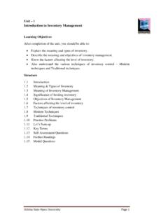
3 Ordering costs: It is the costs that are incurred on obtaining additional inventories. They include costs incurred on communicating the Order , traveling allowance and daily allowance to purchase officers, printing and stationary, salary of purchase department, cost of inspection, cost of receiving the material, transportation cost etc. all above cost, other than transport costs remain unchanged per Order irrespective of the Order size. 2 Dr. Rakesh Kumar Therefore, it is assumed that ordering cost per Order remain constant. The more frequently orders are placed, and fewer the quantities purchased on each Order , the grater will be ordering cost and vice versa. This relation is shown in the figure 1. Carrying cost: It is the cost incurred for holding inventory in hand.

4 They include interest on the money locked up in stocks, storage costs, deterioration spoilage costs, insurance, evaporation, godown rent, pilferage, shrinkage, obsolescence, other overhead of stores department etc. They are assumed to be constant per unit of inventory. The large the volume of inventory, the higher will be the inventory carrying cost and vice versa. This relation is shown in the figure 2. Economic Order Quantity (EOQ) Model 3 From the above discussion it is clear that ordering costs and carrying costs are quite opposite to each other. If we need to minimize carrying costs we have to place small Order which increases the ordering costs. If we want minimize our ordering costs we have to place few orders in a year and this requires placing large orders which in turn increases the total carrying costs for the need to minimize the total inventory costs, Thus EOQ is determine by the intersection of ordering cost curve and carrying cost line.

5 At this point total ordering cost is equal to total carrying cost, and the total of the two costs is the least this is shown in the figure 3. Sensitivity analysis: In sensitivity analysis we take a given scenario and make changes to the variables built into that scenario to establish that the changes made will significantly affect the outcomes. This Model is generally insensitivity to change around the eoq , small error in the numbers to be ordered do not make much difference to the overall result. Mathematical Formulation of EOQ The above graphic method of determining EOQ may not provide the most accurate result. Economic Order Quantity can be calculated mathematically with a great degree of accuracy as given blow: formula EOQ = (2 A O)/C Where, EOQ = Economic Order Quantity 4 Dr.

6 Rakesh Kumar A = Annual demand in units O = Cost incurred to place a single Order C = Carrying cost per unit per year This formula is derived from the following cost function: At EOQ, Total Carrying Cost = Total ordering Cost Carrying cost per unit = C Average inventory = EOQ / 2 Carrying cost of average inventory = (EOQ /2) C Cost incurred to place a single Order = O Order size = EOQ Annual demand in units = A Total number of Order for the period = A / EOQ Total ordering cost for the period = (A / EOQ) O At EOQ, Total Carrying Cost = Total ordering Cost (EOQ /2) C = (A / EOQ) O EOQ EOQ = (2 A O) / C EOQ = (2 A O)/C We can say, Total ordering cost + Total carrying cost = (2 A O C) Assumptions in EOQ Model : The formula is based on the following assumptions. Without these assumptions, the eoq Model cannot work to its optimal potential.

7 1. The demand rate for the year is known and evenly spread throughout the year. 2. There is no time gap between placing an Order and receiving its supply. 3. Ordering cost very directly with the number of orders. 4. Carrying cost very directly with the average inventory. 5. There is no Quantity discount. Limitations of the eoq Model : The assumptions made in the eoq formula restrict the use of the formula . In practice cost per unit of purchase of an item change time to time and lead time are also uncertain. It is necessary for the application of EOQ Order that the demands remain constant throughout the year which is not possible. Ordering cost per Order can t be constant because it s including transport cost. Conclusion the eoq is very useful tool for inventory control it may be applied to finished goods inventories, work-in-progress inventories and raw material inventories.

8 It regulate of purchase and storage of inventory in such a way so as to maintain an even flow of production at the same time avoiding excessive investment in inventories. Economic Order Quantity (EOQ) Model 5 References [1] S. K. Goyal, Economic Order Quantity under Conditions of Permissible Delay in Payments,The Journal of the Operational Research Society, Vol. 36, No. 4 (Apr., 1985), pp. 335-338 [2] Aju Mathew,Demand Forecasting For Economic Order Quantity inInventory Management, International Journal of Scientific and Research Publications, Volume 3, Issue 10, October 2013 [3] Tien-Yu Lin and Ming-Te Chen, An Economic Order Quantity Model with screeningerrors, returned cost, and shortages under quantitydiscounts, African Journal of Business Management Vol. 5(4), pp.

9 1129-1135, 18 February, 2011 [4] Milad Elyasi, Farid Khoshalhan and Mohammad Khanmirzaee,International Journal of Industrial Engineering Computations , Volume 5 Issue 2 pp. 211-222 , 2014 [5] Sarbjit Singh, An Economic Order Quantity Model for Items HavingLinear Demand under Inflation and Permissible Delay,International Journal of Computer Applications (0975 8887)Volume 33 , November 2011 6 Dr. Rakesh Kumar