Transcription of Essential Graphs for Microeconomics
1 Essential Graphs for Microeconomics Basic Economic Concepts Production Possibilities Curve Good X A. B Concepts: Points on the curve-efficient W Points inside the curve-inefficient C Points outside the curve-unattainable with available resources Gains in technology or resources F D favoring one good both not other. E. Good Y. Nature & Functions of Product Markets Demand and Supply: Market clearing equilibrium P. S Variations: Shifts in demand and supply caused by changes in determinants Pe Changes in slope caused by changes in elasticity Effect of Quotas and Tariffs D. Qe Q. Floors and Ceilings P P. S S. Pe Pe D D. QD Qe QS Q QS Qe QD Q. Floor Ceiling Creates surplus Creates shortage Qd<Qs Qd>Qs Consumer and Producer Surplus P. S. Consumer surplus Pe Producer surplus D.
2 Qe Q. Effect of Taxes A tax imposed on the BUYER-demand A tax imposed on the SELLER-supply curve moves left curve moves left elasticity determines whether buyer or elasticity determines whether buyer seller bears incidence of tax or seller bears incidence of tax shaded area is amount of tax shaded area is amount of tax connect the dots to find the triangle connect the dots to find the triangle of deadweight or efficiency loss. of deadweight or efficiency loss. Price Price buyers buyers pay S2. pay P. P. S Price S1. Price w/o w/o tax tax D1 D1. Price Price sellers D2 sellers receive receive Q. Q. Theory of the Firm Short Run cost AFC declines as output increases P/C MC AVC and ATC declines initially, then ATC. reaches a minimum then increases (U- AVC shaped).
3 MC declines sharply, reaches a minimum, the rises sharply MC intersects with AVC and ATC at minimum points When MC> ATC, ATC is falling AFC When MC< ATC, ATC is rising There is no relationship between MC and Q AFC. Long Run cost ATC. Economies Diseconomies of Scale of Scale Constant Returns to Scale Q. Perfectly Competitive Product Market Structure Long run equilibrium for the market and firm-price takers Allocative and productive efficiency at P=MR=MC=min ATC. P MC. S P y Pe Pe MR=D=AR=P. D. Qe Qe Q. Q. Variations: Short run profits , losses and shutdown cases caused by shifts in market demand and supply. Imperfectly Competitive Product Market Structure: Pure Monopoly Single price monopolist (price maker) Natural Regulated Monopoly Earning economic profit Selling at Fair return ( Qfr at Pfr).
4 P. MC. ATC MC. P. Pm ATC. PFR. D PSO. D. Q Q Qm QFR QSO Q. MR MR. Imperfectly Competitive Product Market Structure: Monopolistically Competitive Long run equilibrium where P=AC at MR=MC output MC. P ATC. Variations: PMC Short run profits , losses and shutdown cases caused by shifts in market demand and supply. D. Qmc Q. MR. Factor Market Perfectly Competitive Resource Market Structure Perfectly Competitive Labor Market Wage takers Firm wage comes from market so changes in labor demand do not raise wages. Labor Market Individual Firm S. Wage Wage Rate Rate S = MRC. Wc Wc D = mrp's DL=mrp Qc Quantity qc Quantity Variations: Changes in market demand and supply factors can influence the firm's wage and number of workers hired. Imperfectly Competitive Resource Market Structure Imperfectly Competitive Labor Market Wage makers Quantity derived from MRC=MRP (Qm).
5 Wage (Wm) comes from that point downward to Supply curve. MRC. Wage S. Rate b Wc a Wm MRP. c Qm Qc Q. Market Failures - Externalities MSC Overallocation of resources when external costs are P. present and suppliers are shifting some of their costs onto MPC the community, making their marginal costs lower. The supply does not capture all the costs with the S curve understating total production costs. This means resources D are overallocated to the production of this product. By shifting costs to the consumer, the firm enjoys S1 curve Qo Qe Q and Qe., (optimum output ). Spillover Costs P Underallocation of resources when external S. benefits are present and the market demand curve reflects only the private benefits understating the total benefits. Market demand curve (D) and MSB market supply curve yield Qe.
6 This output will be less MPB than Qo shown by the intersection of D1 and S with resources being underallocated to this use. Qe Qo Q. Spillover Benefits Thinking on the Margin . Allocative Efficiency: Marginal cost (MC) = Marginal Benefit (MB). Definition: Allocative efficiency means that a good's output is expanded until its marginal benefit and marginal cost are equal. No resources beyond that point should be allocated to production. Theory: Resources are efficiently allocated to any product when the MB and MC are equal. Essential Graph: MC MC. The point where MC=MB is &. allocative efficiency since neither underallocation or MB overallocation of resources occurs. MB. Q. Application: External Costs and External Benefits External Costs and Benefits occur when some of the costs or the benefits of the good or service are passed on to parties other than the immediate buyer or seller.
7 MSC External cost P. P MC. MPC External Benefits MB MSB. MPB. Qo Qe Q Qe Qo Q. External costs External benefits production or consumption production or consumption costs costs inflicted on a third party conferred on a third party or without compensation community at large without their pollution of air, water are compensating the producer examples education, vaccinations are examples Supply moves to right Market Demand, reflecting only private producing a larger output that benefits moves to left producing a is socially desirable over smaller output that society would like . allocation of resources under allocation of resources Legislation to stop/limit Legislation to subsidize consumers pollution and specific taxes and/or suppliers and direct production (fines) are ways to correct by government are ways to correct Diminishing Marginal Utility Definition: As a consumer increases consumption of a good or service, the additional usefulness or satisfaction derived from each additional unit of the good or service decreases.
8 Utility is want-satisfying power it is the satisfaction or pleasure one gets from consuming a good or service. This is subjective notion. Total Utility is the total amount of satisfaction or pleasure a person derives from consuming some quantity. Marginal Utility is the extra satisfaction a consumer realizes from an additional unit of that product. Theory: Law of Diminishing Marginal Utility can be stated as the more a specific product consumer obtain, the less they will want more units of the same product. It helps to explain the downward-sloping demand curve. Essential Graph: Total Total Utility increases at a Utility diminishing rate, reaches a maximum and then declines. TU. Unit Consumed Marginal Marginal Utility diminishes with Utility increased consumption, becomes zero where total utility is at a maximum, and is negative when Total Utility declines.
9 MU. Unit When Total Utility is atConsumed its peak, Marginal Utility is becomes zero. Marginal Utility reflects the change in total utility so it is negative when Total Utility declines. Teaching Suggestion: begin lesson with a quick starter by tempting a student with how many candy bars (or whatever) he/she can eat before negative marginal utility sets in when he/she gets sick! Law of Diminishing Returns Definitions: Total Product: total quantity or total output of a good produced Marginal Product: extra output or added product associated with adding a unit of a variable resource change in total product TP. MP =. change in labor input Linput Average Product: the output per unit of input, also called labor productivity total product TP. AP =. units of labor L.
10 Theory: Diminishing Marginal Product a s successive units of a variable resource are added to a fixed resource beyond some point the extra or the marginal product will decline; if more workers are added to a constant amount of capital equipment, output will eventually rise by smaller and smaller amount. Essential Graph: TP. Note that the marginal product intersects the TP average product at its maximum average product. Quantity of Labor Increasing Marginal Returns Negative When the TP has reached it Marginal maximum, the MP is at zero. Returns As TP declines, MP is negative. Diminishing Marginal Returns Quantity of Labor MP. Teaching Suggestion: Use a game by creating a production factory (square off some desks). Start with a stapler, paper and one student.