Transcription of Experimental Uncertainties (Errors) - Purdue University
1 Experimental Uncertainties (Errors). Sources of Experimental Uncertainties ( Experimental Errors): All measurements are subject to some uncertainty as a wide range of errors and inaccuracies can and do happen. Measurements should be made with great care and with careful thought about what you are doing to reduce the possibility of error as much as possible. There are three main sources of Experimental Uncertainties ( Experimental errors): 1. Limited accuracy of the measuring apparatus - , the force sensors that we use in experiment M2 cannot determine applied force with a better accuracy than N. 2. Limitations and simplifications of the Experimental procedure - , we commonly assume that there is no air friction if objects are not moving fast.
2 Strictly speaking, that friction is small but not equal to zero. 3. Uncontrolled changes to the environment. For example: small changes of the temperature and the humidity in the lab. In this laboratory, we keep to a very simple form of error analysis, our purpose being more to raise your awareness of errors than to give you expertise in sophisticated methods for handling error analysis. If you ever need more information on error analysis, please check the literature1-4. In the Analysis section of the lab report, you should identify significant sources of Experimental errors. Do not list all possible sources of errors there. Your goal is to identify only those significant for that experiment! For example, if the lab table is not perfectly leveled, then for the collision experiments (M6 Impulse and Momentum) when the track is supposed to be horizontal, results will have a large, significant error.
3 On the contrary, for the constant acceleration motion on the intentionally inclined track, the table leveling is not going to make a large contribution to the Experimental error. Do not list your mistakes as Experimental errors. These mistakes should have already been detected and eliminated during the preparation of the lab report. A calculator should 1. Bevington, P. R., Data Reduction and Error Analysis for the Physical Sciences, New York: McGraw-Hill, 1969. 2. Taylor, J. R., An introduction to uncertainty analysis: the study of Uncertainties in physical measurements, Mill Valley: University Science Books, 1982. 3. Young, H. D., Statistical Treatment of Experimental data, New York: McGraw-Hill, 1962. 4. Barford N. C., Experimental Measurements: Precision, Error and Truth, Addison-Wesley, 1967.
4 Not be listed as a source of Experimental error. You may always use more significant figures ( the next section) during calculations to reduce round-off error. In other words, you may always make all calculations with a better accuracy then you can do lab measurements. Absolute and Relative Errors: In order to learn the meaning of certain terms, consider an experiment in which we use the ultrasonic motion sensor to measure the position x of an object. The accuracy of the motion sensor has been specified by the manufacturer as 1 mm. The absolute error of our measurements is thus 1 mm. Note that the absolute error carries the same unit as the measured quantity. Suppose the value measured in our first trial was equal to cm. Then the relative error is equal to: (1 mm)/( cm) = ( cm)/( cm) The relative error is dimensionless.
5 It is often expressed in percentage, as: 100%* ( cm)/( cm) We may express the above result using either absolute error or relative error, as follows: x = (cm) (usually preferred) or x = cm If we know the accepted value of the measured quantity ( , the temperature of melting point for water is equal to 0 C or 273K), then we can calculate the percentage error as: Experimental value - Accepted value Relative error = " 100%. Accepted value When comparing Experimental data with the theoretical values, then the relative error is given by a similar formula: ! Experimental value - Theoretical value Relative error = " 100%. Theoretical value If we do not know the accepted value of the measured quantity, but the measurements have been repeated several times for the same conditions, one can use the spread of the !
6 Results themselves to estimate the Experimental error. Average Values and the Standard deviation : Consider the following results of velocity measurements: , , , , , m/s. The average value of these six velocity measurements is equal to: v = ( +. + + + + ) / 6 = m/s. Next, one needs to calculate the deviations from the average velocity: - = m/s; - = m/s; - = m/s; - = m/s; - = m/s; - = m/s. The general formula for calculation of the average value xAV (sometimes also called mean value) is as follows: 1. ( x + x 2 + x 3 + .. + x n ). x AV =. n 1. where n is the number of repeated measurements (for this example n = 6). The values of the deviation from the average value are used to calculate the ! Experimental error. The quantity that is used to estimate these deviations is known as the standard deviation sx and is defined as: 1.
7 Sx =. n "1. ([ 2 2. x1 " x AV ) + ( x 2 " x AV ) + .. + ( x n " x AV ). 2. ]. ! The standard deviation squared - sx2 is the sum of squares of deviations from the average value divided by (n - 1). The subscript usually indicates the quantity that the standard ! deviation is calculated for, , sv stands for the standard deviation of velocity measurements, ! whereas sa is the standard deviation for acceleration data. For the previously discussed example of velocity measurements we have: 1. sv =. 6 "1. [. ( m/s) 2 + ( m/s) 2 + ( m/s) 2 + ( m/s) 2 + ( m/s) 2 + ( m/s) 2 = ]. 1. = # (m2 /s2 ) = m/s $ m/s 5. We use the standard deviation as the value of the Experimental error. The final result of measurements and error analysis should be written as: !
8 V = vAV sv = (m/s) (do not forget to write the appropriate units!). The general format for presenting Experimental results with Experimental error is given by one of the following expressions: final result = average value standard deviation . x = xAV sx units or x = xAV sx (units) or x = (xAV sx) units Obviously, the average value and the standard deviation must have the same units. Agreement Between Two Results: Error estimates are necessary to be able to say whether the two independent measurements of the same thing agree within the stated errors or disagree. For example, two students measured the melting point temperature of ice and obtain results of C and C. Without an estimate of error, we cannot say whether these measurements agree. Suppose the results had been stated with errors: Tmelt = C and Tmelt =.
9 C. Since the first result admits values between C and C and the second between C and C, there is an overlap (between C and C) and the results are in agreement within Experimental errors. C. overlap C. -2 C -1 C 0 C 1 C 2 C. If one cannot find an overlap between the error bands, then the results do not agree with each other. Experimental Uncertainty ( Experimental Error) for a Product of Two Measurements: Sometimes it is necessary to combine two (or even more than two) measurements to get a needed result. A good example is a determination of work done by pulling a cart on an incline that requires measuring the force and the distance independently. Then the value of work can be calculated from a simple formula: W = F s = F x (more precisely: W =.)
10 FAV xAV). Then, the absolute error for work W is given by the following formula: sW = FAV " sx + #x AV " sF , where, sF and sx are standard deviations of force and distance measurements. FAV and xAV. represent average values ! of force and traveled distance, respectively. It is quite common that one of the two measurements is more precise, , has a much smaller standard deviation . In the discussed case of work measurements, we usually know the traveled distance with a much smaller Experimental error, , sx 0. Therefore, we should be able to use the approximate formula: sW " #x AV $ sF. The final result of work measurements should be written as: W = FAV xAV ! sW ( J ) = FAV xAV xAV sF (J). work = average force average distance average distance standard deviation of force (in Joules).