Transcription of Extending Steinberg’s Fatigue Analysis of Electronics ...
1 1 Extending Steinberg s Fatigue Analysis of Electronics Equipment Methodology to a Full Relative Displacement vs. Cycles Curve Revision C By Tom Irvine Email: March 13, 2013 Vibration Fatigue calculations are ballpark calculations given uncertainties in S-N curves, stress concentration factors, natural frequency, damping and other variables. Furthermore, damage increases exponentially with an increase in stress, which magnifies the effect of any error in the stress calculation or in the reference S-N curve. Perhaps the best that can be expected is to calculate the accumulated Fatigue to the correct order-of-magnitude. Introduction Electronic components in vehicles are subjected to shock and vibration environments. The components must be designed and tested accordingly.
2 Dave S. Steinberg s Vibration Analysis for Electronic Equipment is a widely used reference in the aerospace and automotive industries. Steinberg s text gives practical empirical formulas for determining the Fatigue limits for Electronics piece parts mounted on circuit boards. The concern is the bending stress experienced by solder joints and lead wires. The Fatigue limits are given in terms of the maximum allowable 3-sigma relative displacement of the circuit boards for the case of 20 million stress reversal cycles at the circuit board s natural frequency. The vibration is assumed to be steady-state with a gaussian distribution. Note that classical Fatigue methods use stress as the response metric of interest. But Steinberg s approach works in an approximate, empirical sense because the bending stress is proportional to strain, which is in turn proportional to relative displacement.
3 The user then calculates the expected 3-sigma relative displacement for the component of interest and then compares this displacement to the Steinberg limit value. There are several limitations to Steinberg s Fatigue limit method: 1. An electronic component s service life may be well below or well above 20 million cycles. 2 2. A component may undergo nonstationary or non- gaussian random vibration such that its expected 3-sigma relative displacement does not adequately characterize its response to its service environments. 3. The component s circuit board will likely behave as a multi-degree-of-freedom system, with higher modes contributing non-negligible bending stress, and in such a manner that the stress reversal cycle rate is greater than that of the fundamental frequency alone.
4 These obstacles can be overcome by developing a relative displacement vs. cycles curve, similar to an S-N curve. Fortunately, Steinberg has provides the pieces for constructing this RD-N curve, with some assembly required. Note that RD is relative displacement. The Analysis can then be completed using the rainflow cycle counting for the relative displacement response and Miner s accumulated Fatigue equation. Steinberg s Fatigue Limit Equation Figure 1. Component and Lead Wires undergoing Bending Motion L B Z Relative Motion Component h Relative Motion Component Component 3 Let Z be the single-amplitude displacement at the center of the board that will give a Fatigue life of about 20 million stress reversals in a random-vibration environment, based upon the 3 circuit board relative displacement.
5 Steinberg s empirical formula for limit3Z is inches (1) where B = length of the circuit board edge parallel to the component, inches L = length of the electronic component, inches h = circuit board thickness, inches r = relative position factor for the component mounted on the board (Table 1) C = Constant for different types of electronic components (Table 2) < C < Equation (1) is taken from Reference 1. Table 1. Relative Position Factors for Component on Circuit Board r Component Location (Board supported on all sides) 1 When component is at center of PCB (half point X and Y). When component is at half point X and quarter point Y. When component is at quarter point X and quarter point Y. 4 Table 2. Constant for Different Types of Electronic Components C Component Image Axial leaded through hole or surface mounted components, resistors, capacitors, diodes Standard dual inline package (DIP) DIP with side-brazed lead wires 5 Table 2.
6 Constant for Different Types of Electronic Components (continued) C Component Image Through-hole Pin grid array (PGA) with many wires Extending from the bottom surface of the PGA Surface-mounted leadless ceramic chip carrier (LCCC). A hermetically sealed ceramic package. Instead of metal prongs, LCCCs have metallic semicircles (called castellations) on their edges that solder to the pads. Surface-mounted leaded ceramic chip carriers with thermal compression bonded J wires or gull wing wires. 6 Table 2. Constant for Different Types of Electronic Components (continued) C Component Image Surface-mounted ball grid array (BGA). BGA is a surface mount chip carrier that connects to a printed circuit board through a bottom side array of solder balls. Fine-pitch surface mounted axial leads around perimeter of component with four corners bonded to the circuit board to prevent bouncing __ Any component with two parallel rows of wires Extending from the bottom surface, hybrid, PGA, very large scale integrated (VLSI), application specific integrated circuit (ASIC), very high scale integrated circuit (VHSIC), and multichip module (MCM).
7 __ 7 Sample Base Input PSD An RD-N curve will be constructed for a particular case. The resulting curve can then be recalibrated for other cases. Consider a circuit board which behaves as a single-degree-of-freedom system, with a natural frequency of 500 Hz and Q=10. These values are chosen for convenience but are somewhat arbitrary. The system is subjected to the base input shown in Table 3. Table 3. Base Input PSD, GRMS Frequency (Hz) Accel (G^2/Hz) 20 150 2000 The duration will be 1260 seconds, but the response results will be extended as a test to failure. Note that accumulated Fatigue damage for random vibration response increases approximately linearly with increase in duration. The relationship may have some nonlinearity due to the random occurrence of response peaks above 3-sigma.
8 Time History Synthesis The next step is to generate a time history that satisfies the base input PSD in Table 3. The synthesis is performed using the method in Reference 2. The total 1260-second duration is represented as three consecutive 420-second segments. Separate segments are calculated due to computer processing speed and memory limitations. The complete time history set is shown in Figure 2. Each segment essentially has a gaussian distribution, but the histogram plots are also omitted for brevity. The actual histograms have a slight deviation from the gaussian ideal due to the effect of the fade in, but this is incidental. Verification that the complete time history satisfies the PSD specification is shown in Figure 3. 8 Figure 2. -60-40-200204060050100150200250300350400 TIME (SEC)ACCEL (G)SYNTHESIZED TIME HISTORY No.
9 1 GRMS OVERALL-60-40-20020406005010015020025030 0350400 TIME (SEC)ACCEL (G)SYNTHESIZED TIME HISTORY No. 2 GRMS OVERALL-60-40-20020406005010015020025030 0350400 TIME (SEC)ACCEL (G)SYNTHESIZED TIME HISTORY No. 3 GRMS OVERALL 9 Figure 3. Each curve has an overall level of GRMS. The curves are nearly identical. SDOF Response The response Analysis is performed using the ramp invariant digital recursive filtering relationship in Reference 3. The response results are shown in Figure 4. Descriptive statistics are shown in Table 4. History 3 Time History 2 Time History 1 SpecificationFREQUENCY (Hz)ACCEL (G2/Hz)POWER SPECTRAL DENSITY 10 Figure 4. (SEC)REL DISP (INCH)RELATIVE DISPLACEMENT RESPONSE No. 1 fn=500 Hz Q= (SEC)REL DISP (INCH)RELATIVE DISPLACEMENT RESPONSE No.
10 2 fn=500 Hz Q= (SEC)REL DISP (INCH)RELATIVE DISPLACEMENT RESPONSE No. 3 fn=500 Hz Q=10 11 Table 4. Relative Displacement Response Statistics No. 1-sigma (inch) 3-sigma (inch) Kurtosis Crest Factor 1 2 3 Note that the crest factor is the ratio of the peak-to-standard deviation, or peak-to-rms assuming zero mean. Kurtosis is a parameter that describes the shape of a random variable s histogram or its equivalent probability density function (PDF). Rainflow Cycle Counting Table 5. Relative Displacement Results from Rainflow Cycle Counting, Bin Format, Unit: inch, 1260-sec Duration Range Upper Limit Lower Limit Cycle Counts Average Amplitude Max Amp Min Amp Average Mean Max Mean Min Valley Max Peak 12 Next, a rainflow cycle count was performed on the relative displacement time histories using the method in Reference 4.