Transcription of Random Forcing Function and Response - …
1 AN INTRODUCTION TO Random vibration Revision B. By Tom Irvine Email: October 26, 2000. Introduction Random Forcing Function and Response Consider a turbulent airflow passing over an aircraft wing. The turbulent airflow is a Forcing Function . Furthermore, the turbulent pressure at a particular location on the wing varies in a Random manner with time. Direction of Flight Figure 1. For simplicity, consider the aircraft wing to be a single-degree-of-freedom system. The wing would vibrate in a sinusoidal manner if it were disturbed from its rest position and then allowed to vibrate freely.
2 The turbulent airflow, however, forces the wing to undergo a Random vibration Response . Random Base Excitation Consider earthquake motion. The ground vibrates in Random manner during the transient duration. Buildings, bridges, and other structures must be designed to withstand this excitation. An automobile traveling down a rough road is also subjected to Random base excitation. The excitation may become periodic, however, if the road is a "washboard road.". 1. Common Characteristics One common characteristic of these examples is that the motion varies randomly with time.
3 Thus, the amplitude cannot be expressed in terms of a "deterministic" mathematical Function . Dave Steinberg wrote in Reference 1: The most obvious characteristic of Random vibration is that it is nonperiodic. A knowledge of the past history of Random motion is adequate to predict the probability of occurrence of various acceleration and displacement magnitudes, but it is not sufficient to predict the precise magnitude at a specific instant. Frequency Content Pure sinusoidal vibration is composed of a single frequency. On the other hand, Random vibration is composed of a multitude of frequencies.
4 In fact, Random vibration is composed of a continuous spectrum of frequencies. Random vibration is somewhat analogous to white light. White light can be passed through a prism to reveal a continuous spectrum of colors. Likewise, Random vibration can be passed through a spectrum analyzer to reveal a continuous spectrum of frequencies. On the other hand, sinusoidal vibration is analogous to a laser beam, where the light wave is composed of a single frequency. Statistics of a Random vibration Sample A sample Random vibration time history is shown in Figure 2. This time history was "synthesized," or generated analytically.
5 It has the descriptive statistics shown in Table 1. Table 1. Random vibration Descriptive Statistics Parameter Value Duration 4 sec Samples 4000. Mean Std dev G. RMS GRMS. Kurtosis Maximum G. Minimum G. Recall that pure sine vibration has a peak value that is 2 times its RMS value. On the other hand, Random vibration has no fixed ratio between its peak and RMS values. The ratio between the absolute peak and RMS values in Table 1 is 2. G peak = (1). G RMS. Note that the RMS value is equal to the standard deviation value if the mean is zero. The standard deviation is often represented by sigma.
6 Thus, the sample in Figure 2 has a peak value of . A different Random sample could have a higher or lower peak value in terms of its , however. A typical assumption is that Random vibration has a peak value of for design purposes. Again, the example in Figure 2 deviates from this assumption with its peak value of . SAMPLE Random vibration . 5. 4. 3. 2. 1. ACCEL (G). 0. -1. -2. -3. -4. -5. 0 1 2 3 4. TIME (SEC). Figure 2. 3. The time history of Figure 2 is shown again in Figure 3. The amplitude in Figure 3 is scaled in terms of the value. According to theory, the amplitude should be within the 1 limits of the time.
7 SAMPLE Random vibration . 4 . 3 . 2 . 1 . ACCEL. 0. -1 . -2 . -3 . -4 . 0 1 2 3 4. TIME (SEC). Figure 3. Histogram The histogram of the time history in Figure 2 is shown in Figure 4. Note that the histogram of the Random vibration sample has a "bell-shaped" curve. The histogram is an approximate example of a Gaussian or normal distribution. The histogram shows that the Random vibration signal has a tendency to remain near its mean value, which in this case is zero. In contrast, recall the histogram of a sinusoidal signal has the shape of a bathtub. Sine vibration thus tends to remain at its positive and negative peak values.
8 4. For this and other reasons, sine and Random are two very different forms of vibration . There really is no "equivalency" between the two forms, although many engineers have tried to derive a relation. HISTOGRAM OF SAMPLE Random vibration . 1000. 4000 samples total. 900. 800. 700. 600. COUNTS. 500. 400. 300. 200. 100. 0. 0 ACCELERATION (G). Figure 4. Probability Density Function The histogram in Figure 4 can be converted to a "probability density Function ." This would be done by dividing each bar by the total number of samples, 4000 in this case. The resulting Function would be a probability density Function .
9 Furthermore, the amplitude along the X-axis could be represented in terms of . The resulting probability density Function would then approximate a "normal probability density Function .". 5. The equation which characterizes the normal probability Function is well-known. It is available in References 1 and 2. This equation can be integrated to determine the probability that an amplitude will occur inside or outside certain limits. Normal Probability Values Consider a Random vibration time history x(t). Again, the amplitude x(t) cannot be calculated for a given time.
10 Nevertheless, the probability that x(t) is inside or outside of certain limits can be expressed in terms of statistical theory. The probability values for the amplitude are given in Tables 2a and 2b for selected levels in terms of the standard deviation or value. Table 2a. Probability for a Random Signal with Normal Distribution and Zero Mean Statement Probability Ratio Percent Probability - < x < + -2 < x < +2 -3 < x < +3 Table 2b. Probability for a Random Signal with Normal Distribution and Zero Mean Statement Probability Ratio Percent Probability |x|> | x | > 2 | x | > 3 The probability tables can be used as follows.