Transcription of Frequency Response and Bode Plots
1 1 Bob York 2009 1 Frequency Response and Bode Plots Preliminaries The steady-state sinusoidal Frequency - Response of a circuit is described by the phasor transfer function ()Hj . A Bode plot is a graph of the magnitude (in dB) or phase of the transfer function versus Frequency . Of course we can easily program the transfer function into a computer to make such Plots , and for very complicated transfer functions this may be our only recourse. But in many cases the key features of the plot can be quickly sketched by hand using some simple rules that identify the impact of the poles and zeroes in shaping the Frequency Response . The advantage of this approach is the insight it provides on how the circuit elements influence the Frequency Response .
2 This is especially important in the design of Frequency -selective circuits. We will first consider how to generate Bode Plots for simple poles, and then discuss how to handle the general second-order Response . Before doing this, however, it may be helpful to review some properties of transfer functions, the decibel scale, and properties of the log function. Poles, Zeroes, and Stability The s-domain transfer function is always a rational polynomial function of the form 1212 101212 10()()()mmmmmnnnnnsasa sasaNsHs KKDssbsb sbsb ( ) As we have seen already, the polynomials in the numerator and denominator are factored to find the poles and zeroes; these are the values of s that make the numerator or denominator zero. If we write the zeroes as 123,,zz z etc.
3 , and similarly write the poles as 123,,pp p , then ( )Hs can be written in factored form as 1212()( )( )()()( )( )mnszszszHs Kspspsp ( ) 2 Frequency Response and Bode Plots Bob York 2009 The pole and zero locations can be real or complex. When the roots are real they are called simple poles or simple zeros. When the roots are complex they always occur in pairs that are complex conjugates of each other. Another important observation is that stable networks must always have poles and zeroes in the left-half of the complex s-plane, such that the real parts of the poles/zeroes will be negative. As an example, lets assume a stable network with simple poles at 11p and 210p . The transfer function would then be 1211()()()(1)(10)Hsspsps s ( ) Thus for stable networks we always will find terms of the form ()sa in the denominator, where a is a positive number.
4 Students sometimes get confused by the use of ()sp or ()sa to represent the same pole location; just remember that the poles are the values of s that make the denominator zero, sp or sa in this example; clearly these will represent the same pole if pa , and will represent a stable pole if Re{ } 0a or Re{ } 0p . When there are multiple roots at the same location the denominator will contain factors of the form ()rsa , where r is an integer that tells us how many times the root is repeated. For example, a critically-damped second-order Response would have 2r . When the stable network includes a complex-conjugate pole pair, we can represent the pole locations as sj where and are both positive real numbers. The transfer function will then have a factor of the form 22222111()()()2()Hssjsjsss ( ) and thus all the coefficients in the denominator are positive, even though the roots in fact have negative real parts.
5 For reasons which will become clear later it is more convenient to write the second-order polynomial in the standard form 222nnss ( ) where n is called the corner Frequency or break point, and is called the damping factor. Comparing ( ) and ( ) we can relate the corner Frequency and damping factor to the poles using 2222//nn ( ) Decibel Scale and Log Functions Logarithmic scales are useful when plotting functions that vary over many orders of magnitude. This is certainly the case with electrical signals; for example, the signal received by your cell phone is often more than 12 orders of magnitude lower in power than the signal transmitted from the base station!
6 In a filter circuit, the magnitude of the transfer function in the passband may be several orders of magnitude larger than it is in the stop band. We are also interested in the Frequency Response of circuits over a wide range of frequencies, so it makes sense to use a logarithmic scale for frequencies as well as signal intensity. Electrical engineers use the base-ten logarithm function and denote that as log , reserving ln for the natural log function (base e), such that 10logloglnlogexxxx ( ) Preliminaries 3 Bob York 2009 3 This notation is not universal; some computer math programs (such as Mathematica) use Log[x] for the natural log. In order to compute the base-ten log in Mathematica, you have to specify the base by writing Log[10, x].
7 Fortunately all log functions share the following useful properties regardless of base loglogloglog/loglogloglogxABABABAByx y ( ) The bel scale (after inventor Alexander Graham Bell) is defined as the log-base-ten of the ratio of two signal intensities (quantities relating to the power or energy associated with the signal). In circuits work we are often interested in the output-to-input power ratio, /outinPP, but the bel scale can be used to compare any two like quantities (for example, the ratio of signal power to carrier in an AM signal, or the ratio of signal power to noise power in a certain bandwidth). Since there are 10 decibels per bel the power ratio in dB is defined as 1010 log(power ratio in dB)outinPP ( ) Each time the power increases by a factor of ten, the power ratio in dB increases linearly by 10dB.
8 Since power is related to the square of voltage or current, the dB scale for those quantities becomes (assuming identical source and load impedances1) 21010210 log20 log(voltage ratio in dB)outoutininVVVV ( ) In most cases our transfer function is a voltage or current ratio, so we will use 20 log()Hj to compute the magnitude in dB. Some important dB conversions to remember are summarized below: |H| |H|dB 1 20 log 10 dB 2 20 log210 log 2 3 dB 2 20 log 26 dB 4 20 log 412 dB 5 20 log 514 dB 10 20 log 1020 dB A logarithmic scale like the dB scale prove to be a great advantage when dealing with circuit transfer functions, which are always of the form of a rational polynomial function as in ( ). Two related terms we will use in our discussion of Frequency Response Plots are decade and octave.
9 A decade change in Frequency is a factor of ten. So, for example, 1 kHz is a decade above 100 Hz and a decade below 10 kHz. An octave is a factor of two, so similarly 1 kHz is an octave above 500 Hz and an octave below 2 kHz. 1 If the source and load impedances are not the same this shows up as an additive constant in ( ), not especially critical for the discussion of this chapter. 4 Frequency Response and Bode Plots Bob York 2009 Bode Amplitude Plots Simple Poles and Zeroes Consider the transfer function of a first-order circuit with a simple pole at 1s . The AC steady-state Frequency - Response is determined by letting sj 11()( )11 HsH jsj ( ) The magnitude of the transfer function is then given by 1/ 22()1Hj ( ) This function is plotted in Figure 1-1 below for frequencies that are two orders of magnitude above and below 1 ; clearly the Response is quite different on either side of this point.
10 The asymptotic behavior for 1 and 1 can be found from ( ) as dB0 dB1()20 logdB1Hj ( ) These asymptotes are just straight lines on the dB vs. log plot. For 1 the function is a constant, 1H , or 0 dB. At the other extreme where 1 , the transfer function decreases as 20 log in dB; on a log- Frequency scale this is a straight line with a slope of -20 dB/decade; that is, the transfer function decreases by 20dB for every factor of ten increase in Frequency . This slope is equiv-alent to -6dB/octave, a helpful thing to remember. The two straight-line asymptotes capture the essential features of the plot, meeting at a Frequency corresponding to the pole location.