Generalized Linear Models - SAGE Publications Inc

1 15 GeneralizedLinear ModelsDue originally to Nelder and Wedderburn (1972), Generalized Linear Models are a remarkablesynthesis and extension of familiar regression Models such as the Linear Models described inPart II of this text and the logit and probit Models described in the preceding chapter. The currentchapter begins with a consideration of the general structure and range of application of generalizedlinear Models ; proceeds to examine in greater detail Generalized Linear Models for count data,including contingency tables; briefly sketches the statistical theory underlying Generalized linearmodels; and concludes with the extension of regression diagnostics to Generalized Linear unstarred sections of this chapter are perhaps more difficult than the unstarred material inpreceding chapters. Generalized Linear Models have become so central to effective statistical dataanalysis, however, that it is worth the additional effort required to acquire a basic understandingof the The Structure of Generalized Linear ModelsAgeneralized Linear model(or GLM1) consists of three components:1.

2 Arandom component, specifying the conditional distribution of the response variable,Yi(for theith ofnindependently sampled observations), given the values of the explanatoryvariables in the model. In Nelder and Wedderburn s original formulation, the distributionofYiis a member of anexponential family, such as the Gaussian (normal), binomial, Pois-son, gamma, or inverse-Gaussian families of distributions. Subsequent work, however, hasextended GLMs to multivariate exponential families (such as the multinomial distribution ),to certain non-exponential families (such as the two-parameter negative-binomial distribu-tion), and to some situations in which the distribution ofYiis not specified of these ideas are developed later in the Alinear predictor that is a Linear function of regressors i= + 1Xi1+ 2Xi2+ + kXikAs in the Linear model, and in the logit and probit Models of Chapter 14, the regressorsXijareprespecified functions of the explanatory variables and therefore may include quantitativeexplanatory variables, transformations of quantitative explanatory variables, polynomialregressors, dummy regressors, interactions, and so on.

3 Indeed, one of the advantages ofGLMs is that the structure of the Linear predictor is the familiar structure of a Linear A smooth and invertible linearizinglink functiong( ), which transforms the expectation ofthe response variable, i E(Yi), to the Linear predictor:g( i)= i= + 1Xi1+ 2Xi2+ + kXik1 Some authors use the acronym GLM to refer to the generallinear model that is, the Linear regression model withnormal errors described in Part II of the text and instead employ GLIM to denotegeneralizedlinear Models (whichis also the name of a computer program used to fit GLMs).379380 Chapter 15. Generalized Linear ModelsTable Common Link Functions and Their InversesLink i=g( i) i=g 1( i)Identity i iLogloge ie iInverse 1i 1iInverse-square 2i 1/2iSquare-root i 2iLogitloge i1 i11+e iProbit 1( i) ( i)Log-log loge[ loge( i)]exp[ exp( i)]Complementary log-logloge[ loge(1 i)]1 exp[ exp( i)]NOTE: iis the expected value of the response; iis the Linear predictor; and ( )is thecumulative distribution function of the standard-normal the link function is invertible, we can also write i=g 1( i)=g 1( + 1Xi1+ 2Xi2+ + kXik)and, thus, the GLM may be thought of as a Linear model for a transformation of the expectedresponse or as a nonlinear regression model for the response.

4 The inverse linkg 1( )isalso called themean function. Commonly employed link functions and their inverses areshown in Table Note that theidentity linksimply returns its argument unaltered, i=g( i)= i, and thus i=g 1( i)= last four link functions in Table are for binomial data, whereYirepresents theobserved proportion of successes inniindependent binary trials; thus,Yican take onany of the values 0,1/ni,2/ni,.. ,(ni 1)/ni,1. Recall from Chapter 15 that binomialdata also encompass binary data, where all the observations representni=1 trial, andconsequentlyYiis either 0 or 1. The expectation of the response i=E(Yi)is thenthe probability of success, which we symbolized by iin the previous chapter. The logit,probit, log-log, and complementary log-log links are graphed in Figure In contrast tothe logit and probit links (which, as we noted previously, are nearly indistinguishable oncethe variances of the underlying normal and logistic distributions are equated), the log-logand complementary log-log links approach the asymptotes of 0 and 1 the general desire to select a link function that renders the regression ofYon theXs Linear , a promising link will remove restrictions on the range of the expected is a familiar idea from the logit and probit Models discussed in Chapter 14, where theobject was to model the probability of success, represented by iin our current generalnotation.

5 As a probability, iis confined to the unit interval [0,1]. The logit and probit linksmap this interval to the entire real line, from to+ . Similarly, if the responseYis acount, taking on only non-negative integer values, 0, 1, 2,.., and consequently iis anexpected count, which (though not necessarily an integer) is also non-negative, the log linkmaps ito the whole real line. This is not to say that the choice of link function is entirelydetermined by the range of the response the log-log link can be obtained from the complementary log-log link by exchanging the definitions of success and failure, it is common for statistical software to provide only one of the two typically, the complementary The Structure of Generalized Linear Models381 4 ilogitprobitlog logcomplementary log log i = g 1( i)Figure , probit, log-log, and complementary log-log links for binomial data. Thevariances of the normal and logistic distributions have been equated to facilitate thecomparison of the logit and probit links [by graphing the cumulative distributionfunction ofN(0, 2/3) for the probit link].

6 A Generalized Linear model (or GLM) consists of three components:1. A random component, specifying the conditional distribution of the response vari-able,Yi(for theith ofnindependently sampled observations), given the valuesof the explanatory variables in the model. In the initial formulation of GLMs, thedistribution ofYiwas a member of an exponential family, such as the Gaussian,binomial, Poisson, gamma, or inverse-Gaussian families of A Linear predictor that is a Linear function of regressors, i= + 1Xi1+ 2Xi2+ + kXik3. A smooth and invertible linearizing link functiong( ), which transforms the expec-tation of the response variable, i=E(Yi), to the Linear predictor:g( i)= i= + 1Xi1+ 2Xi2+ + kXikA convenient property of distributions in the exponential families is that the conditional varianceofYiis a function of its mean i[say,v( i)] and, possibly, adispersion parameter . The variancefunctions for the commonly used exponential families appear in Table The conditionalvariance of the response in the Gaussian family is a constant, , which is simply alternativenotation for what we previously termed the error variance, 2.

7 In the binomial and Poissonfamilies, the dispersion parameter is set to the fixed value = also shows the range of variation of the response variable in each family, and theso-calledcanonical(or natural )link functionassociated with each family. The canonical link382 Chapter 15. Generalized Linear ModelsTable Link, Response Range, and ConditionalVariance Function for Exponential FamiliesFamilyCanonical Link Range of YiV(Yi| i)GaussianIdentity( ,+ ) BinomialLogit0,1,..,nini i(1 i)niPoissonLog0,1,2,.. iGammaInverse(0, ) 2iInverse-Gaussian Inverse-square(0, ) 3iNOTE: is the dispersion parameter, iis the Linear predictor, and iis the expectation ofYi(the response). In the binomial family,niis thenumber of the GLM,3but other link functions may be used as well. Indeed, one of the strengths ofthe GLM paradigm in contrast to transformations of the response variable in Linear regression is that the choice of linearizing transformation is partly separated from the distribution of theresponse, and the same transformation does not have to both normalize the distribution ofYand make its regression on theXs specific links that may be used vary from onefamily to another and also to a certain extent from one software implementation of GLMs toanother.

8 For example, it would not be promising to use the identity, log, inverse, inverse-square,or square-root links with binomial data, nor would it be sensible to use the logit, probit, log-log,or complementary log-log link with nonbinomial assume that the reader is generally familiar with the Gaussian and binomial families andsimply give their distributions here for reference. The Poisson, gamma, and inverse-Gaussiandistributions are perhaps less familiar, and so I provide some more detail:5 The Gaussian distribution with mean and variance 2has density functionp(y)=1 2 exp (y )22 2 ( ) The binomial distribution for the proportionYof successes innindependent binary trialswith probability of success has probability functionp(y)= nny ny(1 )n(1 y)( )3 This point is pursued in Section is also this more subtle difference: When we transformYand regress the transformed response on theXs, weare modeling the expectation of the transformed response,E[g(Yi)]= + 1xi1+ 2xi2+ + kxikIn a GLM, in contrast, we model the transformed expectation of the response,g[E(Yi)]= + 1xi1+ 2xi2+ + kxikWhile similar in spirit, this is not quite the same thing when (as is true except for the identity link) the link functiong( )is various distributions used in this chapter are described in a general context in Appendix D on probability The Structure of Generalized Linear Models383 Here,nyis the observednumberof successes in thentrials, andn(1 y)is the number offailures; and nny =n!

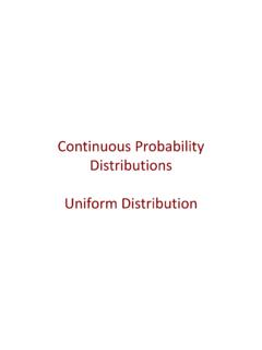
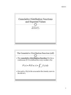
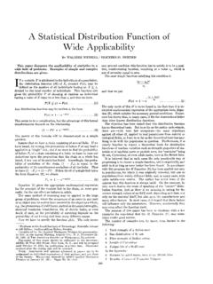
9 (ny)![n(1 y)]!is the binomial coefficient. The Poisson distributions are a discrete family with probability function indexed by therateparameter >0:p(y)= y e y!fory=0,1,2,..The expectation and variance of a Poisson random variable are both equal to . Poissondistributions for several values of the parameter are graphed in Figure As we will seein Section , the Poisson distribution is useful for modeling count data. As increases,the Poisson distribution grows more symmetric and is eventually well approximated by anormal distribution . The gamma distributions are a continuous family with probability-density function indexedby thescale parameter >0 andshape parameter >0:p(y)= y 1 exp y ( )fory>0( )where ( )is the gamma expectation and variance of the gamma distri-bution are, respectively,E(Y)= andV(Y)= 2 . In the context of a generalizedlinear model, where, for the gamma family,V(Y)= 2(recall Table on page 382),the dispersion parameter is simply the inverse of the shape parameter, =1/.

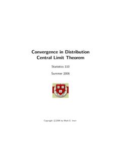
10 Asthenames of the parameters suggest, the scale parameter in the gamma family influences thespread (and, incidentally, the location) but not the shape of the distribution , while the shapeparameter controls the skewness of the distribution . Figure shows gamma distributionsfor scale =1 and several values of the shape parameter . (Altering the scale param-eter would change only the labelling of the horizontal axis in the graph.) As the shapeparameter gets larger, the distribution grows more symmetric. The gamma distribution isuseful for modeling a positive continuous response variable, where the conditional varianceof the response grows with its mean but where thecoefficient of variationof the response,SD(Y )/ , is constant. The inverse-Gaussian distributions are another continuous family indexed by twoparameters, and , with density functionp(y)= 2 y3exp (y )22y 2 fory>0 The expectation and variance ofYareE(Y)= andV(Y)= 3/.