Transcription of GU4204: Statistical Inference
1 GU4204: Statistical InferenceBodhisattva SenColumbia UniversityFebruary 27, 2020 Contents1 Statistical Inference : Motivation .. Recap: Some results from probability .. Back to Example .. Delta method .. Back to Example ..102 Statistical Inference : Statistical model .. Method of Moments estimators ..133 Method of Maximum Properties of MLEs .. Computational methods for approximating MLEs .. s Method .. EM Algorithm ..2214 Principles of Mean squared error .. Comparing estimators .. Unbiased estimators .. Sufficient Statistics ..285 Bayesian Prior distribution .. Posterior distribution .. Bayes Estimators .. Sampling from a normal distribution ..376 The sampling distribution of a The gamma and the 2distributions .. gamma distribution.
2 Chi-squared distribution .. Sampling from a normal population .. Thet-distribution ..457 Confidence intervals468 The (Cramer-Rao) Information Inequality519 Large Sample Properties of the MLE5710 Hypothesis Principles of Hypothesis Testing .. Critical regions and test statistics .. Power function and types of error .. Significance level .. Testing simple hypotheses: optimal tests .. Minimizing theP(Type-II error) .. Uniformly most powerful (UMP) tests .. Thet-test .. Testing hypotheses about the mean with unknown variance .. One-sided alternatives .. Comparing the means of two normal distributions (two-samplettest) One-sided alternatives .. Two-sided alternatives .. the variances of two normal distributions (F-test) .. One-sided alternatives .. Two-sided alternatives .. ratio test.
3 Of tests and confidence sets ..8111 Linear Method of least squares .. Normal equations .. Simple linear regression .. Interpretation .. Estimated regression function .. Properties .. Estimation of 2.. Gauss-Markov theorem .. Normal simple linear regression .. Maximum likelihood estimation .. Inference .. Inference about 1.. Sampling distribution of 0.. Mean response .. Prediction interval .. Inference about both 0and 1simultaneously ..9712 Linear models with normal Basic theory .. Maximum likelihood estimation .. Projections and orthogonality .. Testing hypotheis .. Testing for a component of not included in the final exam .. One-way analysis of variance (ANOVA) .. 10813 The sample distribution function .. The Kolmogorov-Smirnov goodness-of-fit test .. The Kolmogorov-Smirnov test for two samples.
4 Bootstrap .. Bootstrap in general .. Parametric bootstrap .. The nonparametric bootstrap .. 11814 Statistics .. 12041 Statistical Inference : MotivationStatistical inferenceis concerned with makingprobabilistic statementsaboutran-dom variablesencountered in the analysis of : means, median, variances ..Example company sells a certain kind of electronic component. The companyis interested in knowing about how long a component is likely to last on can collect data on many such components that have been used under choose to use the family of exponential distributions1to model the length of time(in years) from when a component is put into service until it company believes that, if they knew the failure rate , thenXn= (X1,X2,..,Xn)would random variables having the exponential distribution with parameter.
5 We may ask the following questions:1. Can weestimate from this data? If so, what is a reasonable estimator?2. Can we quantify the uncertainty in the estimation procedure, , can we con-structconfidence intervalfor ? Recap: Some results from probabilityDefinition 1(Sample mean).Suppose thatX1,X2,.., s with (un-known) mean R( ,E(X1) = ) and variance 2< . A natural estimator of is the sample mean (or average) defined as Xn:=1n(X1+..+Xn) =1nn i= ( Xn) = andVar( Xn) = 2 thatE( Xn) =1nn i=1E(Xi) =1n n = .1 Xhas an exponential distribution with (failure) rate >0, ,X Exp( ), if the ofXis given byf (x) = e x1[0, )(x),forx mean (or expected value) ofXis given byE(X) = 1, and the variance ofXis Var(X) = (1,10) densityHistogram of sample mean when n = of sample mean when n = 1: The plots illustrate the convergence (in probability) of the sample mean tothe population ,Var( Xn) =1n2 Var(n i=1Xi)=1n2 n 2= (Weak law of large numbers).]
6 Suppose thatX1,X2,.., s with finite mean . Then for any >0, we haveP( 1nn i=1Xi E(X) > ) 0asn .This says that if we take the sample average s the sample average willbe close to the true population average. Figure 1 illustrates the result: The leftpanel shows the density of the data generating distribution (in this example we tookX1,.., Exp(10)); the middle and right panels show the distribution (his-togram obtained from 1000 replicates) of Xnforn= 100 andn= 1000, see that as the sample size increases, the distribution of the sample mean concen-trates aroundE(X1) = 1/10 ( , XnP 10 1asn ).Definition 2(Convergence in probability).In the above, we say that the samplemean1n ni=1 Xiconverges in probability to the true (population) generally, we say that the sequence of s{Zn} n=1converges toZin proba-bility, and writeZnP Z,if for every >0,P(|Zn Z|> ) 0asn.
7 This is equivalent to saying that for every >0,limn P(|Zn Z| ) = 3(Convergence in distribution).We say a sequence of s{Zn}ni= sFn( )converges in distributiontoFiflimn Fn(u) =F(u)for allusuch thatFis continuous2atu(hereFis itself a ).The second fundamental result in probability theory, after the law of large numbers(LLN), is the Central limit theorem (CLT), stated below. The CLT gives us theapproximate (asymptotic) distribution of XnTheorem (Central limit theorem).IfX1,X2,..are with mean zero andvariance1, then1 nn i=1 Xid N(0,1),whereN(0,1)is the standard normal distribution. More generally, the usual rescalingtell us that, forX1,X2,..are with mean and variance 2< n( Xn ) 1 nn i=1(Xi )d N(0, 2).The following plots illustrate the CLT: The left, center and right panels of Figure 2show the (scaled) histograms of Xnwhenn= 10,30 and 100, respectively (as before,in this example we tookX1.)
8 , Exp(10); the histograms are obtained from5000 independent replicates). We also overplot the normal density with mean andvariance 10 1/ n. The remarkable agreement between the two densities illustratesthe power of the CLT. Observe that the original distribution of theXi s is skewedand highly nor-normal (Exp(10)), but even forn= 10, the distribution of X10is quiteclose to being class of useful results we will use very much in this course go by the name continuous mapping theorem . Here are two such band ifg( )is a function that is continuous atb, theng(Zn)P g(b).2 Explain why do we need to restrict our attention to continuity points ofF. (Hint: think of thefollowing sequence of distributions:Fn(u) =I(u 1/n), where the indicator function of a setAis one ifx Aand zero otherwise.)It s worth emphasizing that convergence in distribution because it only looks at the is in factweakerthan convergence in probability.
9 For example, ifpXis symmetric, then thesequenceX, X,X, X,..trivially converges in distribution toX, but obviously doesn t convergein , ifU Unif(0,1), then the sequenceU,1 U,U,1 U,..converge in distribution to a uniform distribution. But obviously they do not converge in of sample mean when n = of sample mean when n = of sample mean when n = 2: The plots illustrate the convergence (in distribution) of the sample meanto a normal Zand ifg( )is a function that is continuous, theng(Zn)d g(Z). Back to Example the first example we have the following results: by the LLN, the sample mean Xnconverges in probability to the expectation1/ (failure rate), , XnP 1 ; by the continuous mapping theorem (see Theorem ) X 1nconverges in prob-ability to , , X 1nP ; by the CLT, we know that n( Xn 1)d N(0, 2)where Var(X1) = 2; But how does one find an approximation to the distribution of X 1n?
10 Delta methodThe first thing to note is that if{Zn}ni=1converges in distribution (or probability) toa constant , theng(Zn)d g( ), for any continuous functiong( ).8We can also zoom in to look at the asymptotic distribution (not just the limitpoint) of the sequence of s{g(Zn)}ni=1, wheneverg( ) is sufficiently ,Z2,..,Znbe a sequence of s and letZbe a with acontinuous . Let R, and leta1,a2,.., be a sequence such thatan .Suppose thatan(Zn )d F .Letg( )be a function with a continuous derivative such thatg ( )6= 0. Thenang(Zn) g( )g ( )d F . will only give an outline of the proof (thinkan=n1/2, ifZnas the samplemean). Asan ,Znmust get close to with high probability asn .Asg( ) is continuous,g(Zn) will be close tog( ) with high s sayg( ) has a Taylor expansion around , ,g(Zn) g( ) +g ( )(Zn ),where we have ignored all terms involving (Zn )2and higher ifan(Zn )d Z,for some limit distributionF and a sequence of constantsan , thenang(Zn) g( )g ( ) an(Zn )d F.