Transcription of Introduction to Electrical Systems Modeling
1 Engineering Sciences 22 Systems Electrical Modeling Page 1 Introduction to Electrical Systems Modeling Part I. DC analysis techniques DC analysis techniques are of course important for analyzing DC circuits circuits that are not dynamic. But why do we discuss them in a dynamic Systems class? Firstly, they provide good practice and help build intuition for circuits. Secondly, we will later introduce techniques that allow analyzing many dynamic circuits as if they were simple DC circuits. That will make them really easy to solve if you are proficient with DC circuits. Part I of this document presents the fundamentals of circuit analysis . The information in this section is sufficient to solve any DC circuit. More importantly, it is also essential for Modeling dynamic circuits, and the techniques are presented in a way that makes it directly transferable to analyzing dynamic circuits, as well as nonlinear circuits that you might encounter in an advanced electronics course.
2 Part II presents circuit manipulations techniques shortcuts that make it faster and easier to solve DC circuits. Although the techniques are presented in terms of dc circuits, they are also applicable to dynamic circuits, as you will see in Section III of this handout, and later in the course. Part III introduces dynamic elements and shows how to develop a state-variable model of a dynamic circuit. What s different from what you learned in physics Modeling of Electrical Systems is best approached by thinking separately about the element laws and the interaction laws. The interactions laws are Kirchoff s voltage law (KVL) and Kirchoff s current law (KCL). The element laws are relationships for individual components such as resistors (ohm s law, V = iR), capacitors, inductors, etc. In some textbooks and courses, KVL and the element laws are mixed together KVL is written like v1 iR2 iR3 = 0.
3 That works for simple physics textbooks problems, but it s not really KVL. KVL is actually simpler. It is just a relationship between voltages; for example v1 v6 v5 = 0. Learning to think about the interaction laws and the element laws separately is important because once you learn them separately, you are prepared to deal with any type of problem involving any kind of element configured in any kind of circuit you won t be limited to simple physics-textbook problems. But before we discuss KVL and KCL, we must consider variables to work with and choose sign conventions. Variables Current is the flow of charge. Thinking of current as flow can help you gain intuition about circuits. Charge is measured in coulombs, so its flow is in coulombs/second. Coulombs per second are also called amperes, or amps, abbreviated A. Voltage can be thought of as the force that pushes the flow of charge.
4 In an analogy to a hydraulic system , voltage would correspond to pressure. It is usually pressure differences that matter, not absolute pressure. For voltages, it is always just the voltage difference that matters. Sometimes people will discuss the voltage at a point, without reference to a voltage difference. The only way that can be meaningful is with reference (implicit or explicit) to an arbitrary reference point, which is often called ground. What matters for the operation of circuit elements, however, is just the voltage difference across those elements, not the voltage with respect to an arbitrary reference point. Engineering Sciences 22 Systems Electrical Modeling Page 2 Voltage can also be defined in terms of potential energy of a unit charge. Sign Conventions As in mechanical Systems we must define the sense of each variable we use, and mark that on the diagram (in Electrical Systems , a circuit diagram or schematic).
5 Again, a given arrow or +/- polarity indication does not indicate which way things go; rather, it just indicates which direction we are going to call positive. There is one difference, however. In Electrical Systems , there is a hard and fast rule about the relationship between the two main variables, current and voltage: For any element X (represented by a box here), the signs of voltage and current must be such that positive current is defined flowing from the positive voltage end to the negative voltage end. Actual current and voltage can be in any direction, but the definitions of what s positive must follow this rule. There is one exception: Currents and voltages of sources (voltage sources and current sources) do not need to follow this rule. They may, but it is not required. Fig. 1. Sign conventions for Electrical elements. KVL (Kirchoff s Voltage Law) Kirchoff s voltage law (KVL) states that if you follow any closed loop around a circuit, the sum of voltage drops across each element must sum to zero.
6 =loopclosednv0 where vn is the voltage across some element n. In this sum, add voltage positively, if, in going around the loop, you go up in voltage when you hit that element. That is, if you go from minus to plus in that element s voltage indication. Subtract it if you go down that is, from plus to minus. (Actually you can follow any consistent convention you want, but the one described makes the most physical sense.) Kirchoff s voltage law is often explained in terms of conservation of energy, but it is also very simply a consequence of the fact that the voltage for an element is defined as a voltage difference; it is an inevitable consequence of that definition independent of any physics. (Where the physics comes is in showing that it is possible to uniquely define a voltage difference between two points.) X XXX + VX - - VX ++ VX-- VX + IXIX IXIXV alid current and voltage definitions X XXX + VX - - VX ++ VX-- VX + IXIX IXIXI ncorrect current and voltage definitions Engineering Sciences 22 Systems Electrical Modeling Page 3 The definition above is all you need to know to apply KVL.
7 You can follow the algorithm described and generate KVL equations for any circuit, without any further thought. However, for the reader who would like to have a better understanding of what it is really about, rather than just a rule to follow by rote, some way to visualize voltage and KVL is helpful. One way to visualize voltage is as a height. This makes Electrical potential analogous to gravitational potential, which is necessarily proportional to height (in a contant gravitational field.) For example, consider the following circuit, containing four elements. The elements are drawn as boxes to indicate that they could be any circuit elements. (The differences between circuit elements will be taken into account in their element laws; they don t matter at all for KVL.) Fig. 2. Example circuit with four generic elements. Before we go any futher, we should define variables; since we are only discussing KVL, we need only definitions of voltages.
8 They can be defined in any polarity. Once choice is shown below. Fig. 3. Example circuit with voltage variables defined. For simplicity, let s consider the case in which all the variables, v1 through v4, are positive numbers. To visualize this, first let s lay out the circuit in the first two dimensions of a three-dimensional space: Fig. 4 Example circuit laid out in two dimensions of a 3-D space. 0 5 10 voltage - v1 +- v3 ++v4 - +v2 - Engineering Sciences 22 Systems Electrical Modeling Page 4 Now we turn on the power and use the third dimension to indicate voltage. Fig. 5. Example circuit with voltage shown in the third dimension. Consider KVL from this diagram. We can start at any point. Starting at the base of element 2, we go up by v2. Then we go up by v3. The running total becomes v2 + v3 . Then we go down by v4 and finally down by v1.
9 The total around the loop is v2 + v3 - v4 - v1 = 0 (1) The sum around the loop must be equal to zero because we come back to the starting point, marked as zero volts. In order to draw this example, we had to assume particular values of the voltages; these were v2 = 8 V, v3 = 2 V, v4 = 7 V, and v1 = 3 V. However, we did not need those assumptions in order to write KVL (1). We could have written that simply from looking at Fig. 3. Starting from the same point and going around the loop clockwise, we go to + on element 2 (+), to + on element 3 (+), + to on element 4 ( ), and + to on element 1 ( ), which gives the same KVL equation (1). Since (1) can be derived independent of the numerical values for the voltages (v1 through v4), it ought to work just fine regardless of the values of the voltage, and regardless of their signs. Fig. 6 shows the same circuit with the same definitions of the voltage variables, but with different values for those voltages.
10 + v1 - 0 5 10 voltage + v4 - + v2 - + v3 - Engineering Sciences 22 Systems Electrical Modeling Page 5 Fig. 6 The same circuit at a different point in time, when the voltages take on different values. Here, v3 is negative, as can be seen from the fact that its (+) end is below its ( ) end. More precisely, the voltages are v2 = 10 V, v3 = -4 V, v4 = 3 V, and v1 = 3 V. To confirm that the same KVL equation (1) holds, we can plug in the numbers: 10 V ( 4 V) 3 V 3 V = 0 As stated under Sign Conventions, a given +/- polarity indication does not indicate the actual polarity; rather, it just indicates which direction is called positive. Here the actual state of the circuit is opposite the direction of the polarity indication. The variable v3 is a negative number, but that doesn t matter for KVL.