Transcription of Introduction to Machine Learning - arXiv
1 Introduction to Machine Learning67577 - Fall, 2008 Amnon ShashuaSchool of Computer Science and EngineeringThe Hebrew University of JerusalemJerusalem, [ ] 23 Apr 2009 Contents1 Bayesian Decision Example: Coin Example: Gaussian Density Bayes Classifier for 2-class Normal Distributions102 Maximum Likelihood/ Maximum Entropy and Empirical Entropy and Duality ML/MaxEnt153EM Algorithm: ML over Mixture of EM Algorithm: with to the Coins Gaussian Mixture and Multinomial Mixture and bag of words Application 274 Support Vector Machines and Kernel Margin Classifier as a Quadratic Linear Programming Support Vector Kernel The Homogeneous Polynomial The non-homogeneous Polynomial The RBF Classifying New Instances39iiiivContents5 Spectral Analysis I: PCA, LDA, : Statistical Maximizing the Variance of Output Decorrelation: Diagonalization of the : Optimal Casen >> s LDA: Basic s LDA: General s LDA: versus Correlation Analysis556 Spectral Analysis II: Algorithm for Matrix Formulation of Clustering.
2 Ratio-Cuts and Normalized-Cuts657 The Formal (PAC) Learning Formal Rectangle Learning of Finite Concept The Realizable The Unrealizable Case778 The VC VC Relation between VC dimension and PAC Learning859 The Double-Sampling Polynomial Bound on the Sample Sizemfor of SVM Revisited9510 Appendix97 Bibliography1051 Bayesian Decision TheoryDuring the next few lectures we will be looking at the inference from trainingdata problem as arandomprocess modeled by the joint probability distribu-tion over input (measurements) and output (say class labels) variables. Ingeneral, estimating the underlying distribution is a daunting and unwieldytask, but there are a number of constraints or tricks of the trade so tospeak that under certain conditions make this task manageable and make things simple, we will assume a discrete world, , that thevalues of our random variables take on a finite number of values.
3 Considerfor example two random variablesXtaking onkpossible valuesx1,..,xkandHtaking on two valuesh1,h2. The values ofXcould stand for a BodyMass Index (BMI) measurementweight/height2of a person andHstandsfor the two possibilitiesh1standing for the person being over-weight andh2as the possibility person of normal weight . Given a BMI measurementwe would like to estimate the probability of the person being joint probabilityP(X,H) is a two dimensional array (2-way array)with 2kentries (cells). Each training example (xi,hj) falls into one of thosecells, thereforeP(X=xi,H=hj) =P(xi,hj) holds the ratio between thenumber of hits into cell (i,j) and the total number of training examples(assuming the training data arrive ).
4 As a result ijP(xi,hj) = projections of the array onto its vertical and horizontal axes by sum-ming over columns or over rows is calledmarginalizationand producesP(hj) = iP(xi,hj) the sum over the j th row is the probabilityP(H=hj), , the probability of a person being over-weight (or not) before we see anymeasurement these are calledpriors. Likewise,P(xi) = jP(xi,hj)is the probabilityP(X=xi) which is the probability of receiving sucha BMI measurement to begin with this is often calledevidence. Note12 Bayesian Decision Theoryh125421h200332x1x2x3x4x5 Fig. Joint probabilityP(X,H) whereXranges over 5 discrete values andHover two values. Each entry contains the number of hits for the cell (xi,hj).
5 Thejoint probabilityP(xi,hj) is the number of hits divided by the total number of hits(22). See text for more , by definition, jP(hj) = iP(xi) = 1. In Fig. we have thatP(h1) = 14/22,P(h2) = 8/22 that is there is a higher prior probability of aperson being over-weight than being of normal weight. AlsoP(x3) = 7/22is the highest meaning that we encounter BMI =x3with the highest probabilityP(hj|xi) =P(xi,hj)/P(xi) is the ratio be-tween the number of hits in cell (i,j) and the number of hits in the i thcolumn, , the probability that the outcome isH=hjgiven the measure-mentX=xi. In Fig. we haveP(h2|x3) = 3/7. Note that jP(hj|xi) = jP(xi,hj)P(xi)=1P(xi) jP(xi,hj) =P(xi)/P(xi) = , the conditional probabilityP(xi|hj) =P(xi,hj)/P(hj) is thenumber of hits in cell (i,j) normalized by the number of hits in the j th rowand represents the probability of receiving BMI =xigiven the class labelH=hj(over-weight or not) of the person.
6 In Fig. we haveP(x3|h2) =3/8 which is the probability of receiving BMI =x3given that the person isknown to be of normal weight. Note that iP(xi|hj) = Bayes formula arises from:P(xi|hj)P(hj) =P(xi,hj) =P(hj|xi)P(xi),from which we get:P(hj|xi) =P(xi|hj)P(hj)P(xi).The left hand sideP(hj|xi) is called theposteriorprobability andP(xi|hj)is called theclass conditional likelihood. The Bayes formula provides away to estimate the posterior probability from the prior, evidence and classlikelihood. It is useful in cases where it is natural to compute (or collectdata of) the class likelihood, yet it is not quite simple to compute directlyBayesian Decision Theory3the posterior. For example, given a measurement 12 we would like toestimate the probability that the measurement came from tossing a pairof dice or from spinning a roulette table.
7 Ifx= 12 is our measurement,andh1stands for pair of dice andh2for roulette then it is naturalto compute the class conditional:P( 12 | pair of dice ) = 1/36 andP( 12 | roulette ) = 1/38. Computing the posterior directly is muchmore difficult. As another example, consider medical diagnosis. Once it isknown that a patient suffers from some diseasehj, it is natural to evaluatethe probabilitiesP(xi|hj) of the emerging symptomsxi. As a result, inmany inference problems it is natural to use the class conditionals as thebasic building blocks and use the Bayes formula to invert those to obtainthe Bayes rule can often lead to unintuitive results the one in particu-lar is known as base rate fallacy which shows how an nonuniform prior caninfluence the mapping from likelihoods to posteriors.
8 On an intuitive basis,people tend to ignore priors and equate likelihoods to posteriors. The follow-ing example is typical: consider the Cancer test kit problem which has thefollowing features: given that the subject has Cancer C , the probabilityof the test kit producing a positive decision + isP(+|C) = (whichmeans thatP( |C) = ) and the probability of the kit producing a neg-ative decision - given that the subject is healthy H isP( |H) = (which means also thatP(+|H) = ). The prior probability of Cancerin the population isP(C) = These numbers appear at first glanceas quite reasonable, , there is a probability of 98% that the test kit willproduce the correct indication given that the subject has Cancer.
9 Whatwe are actually interested in is the probability that the subject has Cancergiven that the test kit generated a positive decision, ,P(C|+). UsingBayes rule:P(C|+) =P(+|C)P(C)P(+)=P(+|C)P(C)P(+|C)P(C) +P(+|H)P(H)= means that there is a chance that the subject has Cancer giventhat the test kit produced a positive response by all means a very we draw the posteriorsP(h1|x) andP(h2|x) using the probabilitydistribution array in Fig. we will see thatP(h1|x)> P(h2|x) for allvalues ofXsmaller than a value which is in betweenx3andx4. Thereforethe decision which will minimize the probability of misclassification would This example is adopted from Yishai Mansour s class notes on Machine Decision Theorybe to choose the class with the maximal posterior:h = argmaxjP(hj|x),which is known as the Maximal A Posteriori (MAP) decision principle.
10 SinceP(x) is simply a normalization factor, the MAP principle is equivalent to:h = argmaxjP(x|hj)P(hj).In the case where information about the priorP(h) is not known or it isknown that the prior is uniform, the we obtain the Maximum Likelihood(ML) principle:h = argmaxjP(x|hj).The MAP principle is a particular case of a more general principle, knownas proper Bayes , where alossis incorporated into the decision (hi,hj) be the loss incurred by deciding on classhiwhen in facthjisthe correct class. For example, the 0/1 loss function is:l(hi,hj) ={1i6=j0i=j}The least-squares loss function is:l(hi,hj) = hi hj 2typically used whenthe outcomes are vectors in some high dimensional space rather than classlabels.
![arXiv:0706.3639v1 [cs.AI] 25 Jun 2007](/cache/preview/4/1/3/9/3/1/4/b/thumb-4139314b93ef86b7b4c2d05ebcc88e46.jpg)
![arXiv:1301.3781v3 [cs.CL] 7 Sep 2013](/cache/preview/4/d/5/0/4/3/4/0/thumb-4d504340120163c0bdf3f4678d8d217f.jpg)
![@google.com arXiv:1609.03499v2 [cs.SD] 19 Sep 2016](/cache/preview/c/3/4/9/4/6/9/b/thumb-c349469b499107d21e221f2ac908f8b2.jpg)