Transcription of Introduction to Time Series Regression and …
1 14-1 Introduction to time Series Regression and forecasting (SW Chapter 14) time Series data are data collected on the same observational unit at multiple time periods Aggregate consumption and GDP for a country (for example, 20 years of quarterly observations = 80 observations) Yen/$, pound/$ and Euro/$ exchange rates (daily data for 1 year = 365 observations) Cigarette consumption per capita in a state, by year 14-2 Example #1 of time Series data: US rate of price inflation, as measured by the quarterly percentage change in the Consumer Price Index (CPI), at an annual rate 14-3 Example #2: US rate of unemployment 14-4 Why use time Series data?
2 To develop forecasting models o What will the rate of inflation be next year? To estimate dynamic causal effects o If the Fed increases the Federal Funds rate now, what will be the effect on the rates of inflation and unemployment in 3 months? in 12 months? o What is the effect over time on cigarette consumption of a hike in the cigarette tax? Or, because that is your only option .. o Rates of inflation and unemployment in the US can be observed only over time ! 14-5 time Series data raises new technical issues time lags Correlation over time (serial correlation, autocorrelation) forecasting models built on Regression methods.
3 O autoregressive (AR) models o autoregressive distributed lag (ADL) models o need not (typically do not) have a causal interpretation Conditions under which dynamic effects can be estimated, and how to estimate them Calculation of standard errors when the errors are serially correlated 14-6 Using Regression Models for forecasting (SW Section ) forecasting and estimation of causal effects are quite different objectives. For forecasting , o 2R matters (a lot!) o Omitted variable bias isn t a problem! o We will not worry about interpreting coefficients in forecasting models o External validity is paramount: the model estimated using historical data must hold into the (near) future 14-7 Introduction to time Series Data and Serial Correlation (SW Section ) First, some notation and terminology.
4 Notation for time Series data Yt = value of Y in period t. Data set: Y1,..,YT = T observations on the time Series random variable Y We consider only consecutive, evenly-spaced observations (for example, monthly, 1960 to 1999, no missing months) (missing and non-evenly spaced data introduce technical complications) 14-8We will transform time Series variables using lags, first differences, logarithms, & growth rates 14-9 Example: Quarterly rate of inflation at an annual rate ( ) CPI = Consumer Price Index (Bureau of Labor Statistics) CPI in the first quarter of 2004 (2004.)
5 I) = CPI in the second quarter of 2004 (2004:II) = Percentage change in CPI, 2004:I to 2004:II = = = Percentage change in CPI, 2004:I to 2004:II, at an annual rate = 4 = (percent per year) Like interest rates, inflation rates are (as a matter of convention) reported at an annual rate. Using the logarithmic approximation to percent changes yields 4 100 [log( ) log( )] = 14-10 Example: US CPI inflation its first lag and its change 14-11 Autocorrelation The correlation of a Series with its own lagged values is called autocorrelation or serial correlation.
6 The first autocorrelation of Yt is corr(Yt,Yt 1) The first autocovariance of Yt is cov(Yt,Yt 1) Thus corr(Yt,Yt 1) = 11cov( ,)var( ) var()ttttYYYY = 1 These are population correlations they describe the population joint distribution of (Yt, Yt 1) 14-12 14-13 Sample autocorrelations The jth sample autocorrelation is an estimate of the jth population autocorrelation: j = cov( ,)var( )ttjtYYY where cov( ,)ttjYY = 1,1,11()( )TtjTtj TjtjYYY YT where 1,jTY is the sample average of Yt computed over observations t = j+1.
7 ,T. NOTE: o the summation is over t=j+1 to T (why?) o The divisor is T, not T j (this is the conventional definition used for time Series data) 14-14 Example: Autocorrelations of: (1) the quarterly rate of inflation (2) the quarter-to-quarter change in the quarterly rate of inflation 14-15 The inflation rate is highly serially correlated ( 1 = .84) Last quarter s inflation rate contains much information about this quarter s inflation rate The plot is dominated by multiyear swings But there are still surprise movements!
8 14-16 Other economic time Series : 14-17 Other economic time Series , ctd: 14-18 Stationarity: a key requirement for external validity of time Series Regression Stationarity says that history is relevant: For now, assume that Yt is stationary (we return to this later). 14-19 Autoregressions (SW Section ) A natural starting point for a forecasting model is to use past values of Y (that is, Yt 1, Yt 2,..) to forecast Yt. An autoregression is a Regression model in which Yt is regressed against its own lagged values. The number of lags used as regressors is called the order of the autoregression.
9 O In a first order autoregression, Yt is regressed against Yt 1 o In a pth order autoregression, Yt is regressed against Yt 1,Yt 2,..,Yt p. 14-20 The First Order Autoregressive (AR(1)) Model The population AR(1) model is Yt = 0 + 1Yt 1 + ut 0 and 1 do not have causal interpretations if 1 = 0, Yt 1 is not useful for forecasting Yt The AR(1) model can be estimated by OLS Regression of Yt against Yt 1 Testing 1 = 0 v. 1 0 provides a test of the hypothesis that Yt 1 is not useful for forecasting Yt 14-21 Example: AR(1) model of the change in inflation Estimated using data from 1962:I 2004:IV: tInf = Inft 1 2R = ( ) ( ) Is the lagged change in inflation a useful predictor of the current change in inflation?
10 T = .238/.096 = > (in absolute value) Reject H0: 1 = 0 at the 5% significance level Yes, the lagged change in inflation is a useful predictor of current change in inflation but the 2R is pretty low! 14-22 Example: AR(1) model of inflation STATA First, let STATA know you are using time Series data generate time =q(1959q1)+_n-1; _n is the observation no. So this command creates a new variable time that has a special quarterly date format format time %tq; Specify the quarterly date format sort time ; Sort by time tsset time ; Let STATA know that the variable time is the variable you want to indicate the time scale 14-23 Example: AR(1) model of inflation STATA, ctd.