Sales Prediction with Time Series Modeling - …

1 Sales Prediction with time Series Modeling Gautam Shine, Sanjib Basak I. Introduction Predicting Sales -related time Series quantities like number of transactions, page views, and revenues is important for retail companies. Our work focuses on the revenue data for a US-based online retail company (Digital River, Inc.) that is responsible for the ecommerce platform of its clients. As online Sales are increasing at a massive rate, accurate Prediction of Sales allows the company to properly prepare for handling the shocks to product stock, website traffic, and customer support. During the 3 biggest days Thanksgiving, Black Friday and Cyber Monday the company earns about 10% of the revenue of the whole year, so it is considered a leading indicator of overall Sales . Predicting revenue on special days such as this is especially challenging, as those are usually large spikes ( anomalies) compared to normal days. For example, gross Sales on Black Friday are usually more than 10 times of the median Sales of the year.

2 Our data was limited to only 2-3 years of Black Friday, Cyber Monday, and holiday season Sales data so building a robust model is difficult because these special incidents have only a few data points. II. Data and Prior Work time Series forecasting grew out of econometrics and involves parameter fitting using data to predict future values of some quantity. The input data consists of pairs (rt, t) of some quantity r at time t. Unlike the observations prevalent in most of machine learning, time Series data points are emphatically not independent, and in fact we rely on their autocorrelation structure to forecast the future. Traditional forecasting tools are based on autoregression (AR) and moving averages (MA), which are described below. In addition to these, we will use feed-forward artificial neural networks with time Series inputs to see how they perform. In principle, neural nets have greater freedom to handle nonlinearities, but they are also non-convex black boxes while AR and MA have the advantage of being interpretable and parsimonious because they are specific to time Series .

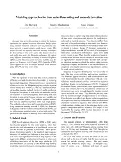
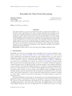
3 Neural nets were popular for time Series forecasting in the 1990 s, but interest died down due to mixed results relative to AR and MA models [1][2]. They have been used specifically for Sales forecasting with some success [3][4]. The data we will use for forecasting has been taken for one large client of Digital River from April 2013 until the present. For this data set itself, prior predictions by the company have been carried out by moving averages, which have low accuracy. Na ve seasonal methods have also been used, which gives decent accuracy but no dynamism since it s merely repeating the prior year s observations. We will attempt to use learning and Prediction to forecast this Series , with particular attention to the distinctive spikes in Sales on holidays. Fig. 1 time Series Sales data used in this work III. Methods and Features Autoregressive integrated moving average (ARIMA) The baseline time Series Modeling methods are [5]: 1.

4 Autoregression (AR): the output at time t is a linear combination of past outputs != + !+ !!! !!!!!!! 2. Moving average (MA): the output at time t is a linear combination of past shocks (noise terms) != + !+ !!! !!!!!!! AR and MA can be combined. They can also be applied to the differenced Series ( an approximation to the derivative) of the desired order and integrated to retrieve the original Series . Putting these three features together yields the more general Autoregressive Integrated Moving Average (ARIMA) model: != + !+ !!! !!!!!!!+ !!! !!!!!!! The order (p,d,q) of the ARIMA model specifies the number of autoregression lags, order of differencing, number of moving average lags, respectively. Our model chose these parameters based on the Akaike information criterion (AIC), which trades off the likelihood of the model against the number of parameters. It is therefore a regularized maximum likelihood estimate and theoretically minimizes 1-step MSE.

5 Because we have multiple seasonality components and discrete spikes in the data to deal with , we have used ARIMA with additional regressors. One set of regressors are the first 3 to 15 largest Fourier components for weekly and yearly seasonality. The other set are indicator vectors that are 0 throughout the year except for 1 s on certain special days like Thanksgiving, Black Friday, and Christmas. The latter is necessary (rather than simply using the input !!!"#) because some of these days change dates every year ( always on a Friday) and because of leap years. Seasonal and Trend decomposition using Loess (STL) STL Decomposition is a useful tool for accounting for seasonal effects. In Sales data, it is common to have repeating patterns every 24 hours, or every 7 days, or every 365 days due to work/sleep cycles and holidays. It is beneficial to remove these consistent fluctuations so that the model parameters have greater freedom to fit any underlying trends, broad changes, and then add the periodic pattern back in as a post-processing step.

6 Both our ARIMA and neural net models made use of STL decomposition. Feed-forward Neural Networks (FFNN) A feed-forward neural network weights its inputs and feeds them into hidden layers that apply some function to these internal inputs. The input yj into the jth hidden layer is: != !+ !" !!!!! After which yj is transformed using a sigmoidal function for categorical or probability outputs or a linear function for regression outputs, which is applicable to our case. The parameters bj and wij are learned from the data and used to make future predictions. Fig. 2 shows a visualization of one of the actual neural networks used in this work, with the line thicknesses encoding the trained weight parameter values. In order to predict time Series , an autoregression component can be included into neural nets by feeding in lagged values of the Series . Without the hidden layer, a neural net with inputs rt rt-1 .. rt-p is equivalent to an AR(p), autoregression of order p.

7 The inclusion of the hidden layer induces nonlinearity that could potentially allow the neural net to surpass ARIMA. As with the ARIMA model, we used holiday indicator vectors as regressors in addition to the lagged time Series . IV. Results Our 390-day Sales forecast is shown above for an ARIMA(5,2,0) model and a neural net with 10 autoregression lagged inputs, 5 indicator vectors for special days, and 14 hidden nodes. The ARIMA model had a higher mean square error (MSE) of 59 to the neural net s 49, but their failures are similar. I1I2I3I4I5I6I7I8I9I10I11I12I13I14I15I16I 17I18I19I20I21I22I23X2X3X4X5X6X7X8X9X10X 11X12X13X14X15X16X17X18X19X20X21X22X23X2 4H1H2H3H4H5H6H7H8H9H10H11O1X1B1B20100200 3000510 1520 25 30 Neural Net: 10 26 N/ATime (Days) Sales (Million USD)01002003000510 1520 25 30 ARIMA: 5 2 0 time (Days) Sales (Million USD)ARIMA Order (5,2,0) Neural Network 14 Hidden Nodes Predicted Actual Predicted Actual Fig.

8 2 Feed-forward neural network with 23 inputs and 11 hidden layers Fig. 3 Sales forecasts using ARIMA (left) and neural nets (right) Both severely underpredict holiday Sales , particularly the Black Friday to Cyber Monday spike. While the neural net successfully captures its discrete nature, the ARIMA model smoothly goes up then down, as expected from its equations. The notable spike at around day 320 highlights the difficulty of this Prediction task: this particular jump in Sales was induced by a hyped-up new product launch and thus could not have been predicted using any of our input features. A hypothetical feature vector to handle this would need to be trained on previous product launches and needs to somehow encode the event into a representative number. Since the neural net can qualitatively capture the holiday spike, it would be interesting to combine linear regression with holiday indicator variables into the ARIMA equation to capture the same effect.

9 Fig. 4 shows such a model, where the optimal order has now changed to (4,1,0) per the AIC criterion and the MSE decreased further to 34. Parameter Fitting in Neural Nets The neural net optimization problem is non-convex when there are one or more hidden layers, so the solution lands in a local optimum almost every time and differs for different initial parameters. We used 100 runs of the neural net initialized randomly using different seed values and averaged the predictions. The number of hidden nodes was chosen by test error minimization, but the caveat is that the actual MSE was close in magnitude to similar models and all of them are ensemble local optima solutions so it s possible the true global minimum is not at our chosen value of 14. The order of autoregression was similarly chosen by minimizing test MSE, but we found that beyond 5 terms made little additional difference. The same caveat applies, although the anticipated effect is small since MSE values did not differ much.

10 510152025305060708090100 MSE v. Hidden NodesNumber of Hidden NodesMean Square Error01002003000510 1520 25 30 ARIMA: 4 1 0 time (Days) Sales (Million USD)ARIMA Order (4,1,0) + Regression Fig. 4 Sales forecast using ARIMA with regression Predicted Actual Fig. 5 Test MSE against hidden node count The learning curve for our time Series data is shown in Fig. 6. The curves are non-monotonic since different set sizes entail different forecast intervals and some parts of the Series are more difficult to capture. Nevertheless, we can observe that neural nets have much higher generalization error for low training set sizes but become roughly comparable as the set size increases. Discussion and Future Work Pure black box time Series Prediction can only do well under limited circumstances, such as highly seasonal data with no long-term changes. The greatest improvement to our models could come from the use of domain knowledge to construct highly relevant regressors that can account for discrete events ( a product release) or long-term changes ( company or economy is on the upswing).