Stock Trading with Recurrent Reinforcement …

1 Stock Trading with Recurrent Reinforcement learning (RRL)CS229 Application ProjectGabriel molina , SUID 50557831I. INTRODUCTIONOne relatively new approach to financial Trading is to use machine learning algorithms to predict the rise and fall ofasset prices before they occur. An optimal trader would buy an asset before the price rises, and sell the asset before its value declines. For this project, an asset trader will be implemented using Recurrent Reinforcement learning (RRL). The algorithm and its parameters are from a paper written by Moody and Saffell1. It is a gradient ascent algorithm which attemptsto maximize a utility function known as Sharpe s ratio. By choosing an optimal parameterwfor the trader, we attempt to take advantage of asset price changes.

2 Test examples of the asset trader s operation, both real-world and contrived, are illustrated in the final UTILITY FUNCTION: SHARPE S RATIOOne commonly used metric in financial engineering is Sharpe s ratio. For a time series of investment returns, Sharpe s ratio can be calculated as: )()(ttTRDeviationStandardRAverageS for interval ,1, twhere tR is the return on investment for Trading periodt. Intuitively, Sharpe s ratio rewards investment strategies that rely on less volatile trends to make a TRADER FUNCTIONThe trader will attempt to maximize Sharpe s ratio for a given price time series. For this project, the trader function takes the form of a neuron:)tanh(ttxwF whereMis the number of time series inputs to the trader, the parameter2 Mw, the input vector 1.

3 ,,1 tMtttFrrx, and the return 1 tttppr. Note that tr is the difference in value of the asset between the current period t and the previous period. Therefore,tr is the return on one share of the asset bought at time 1 t. Also, the function ]1,1[ tF represents the Trading position at timet. There are three types of positions that can be held: long, short, or neutral. A long position is when0 tF. In this case, the trader buys an asset at price tpand hopes that it appreciates byperiod1 short position is when0 tF. In this case, the trader sells an asset which it does not own at pricetp, with the expectation to produce the shares at period1 t. If the price at 1 tis higher, then the trader is forced to buy at the higher1 t price to fulfill the contract.

4 If the price at 1 t is lower, then the trader has made a profit. 1 J Moody, M Saffell, learning to Trade via Direct Reinforcement , IEEE Transactions on Neural Networks, Vol 12, No 4, July neutral position is when 0 tF. In this case, the outcome at time 1 thas no effect on the trader s profits. There will be neither gain nor ,tFrepresents holdings at period t. That is, ttFn shares are bought (long position) or sold (short position), where is the maximum possible number of shares per transaction. The return at time t, considering the decision1 tF, is: 11 tttttFFrFR where is the cost for a transaction at period t. If 1 ttFF ( no change in our investment this period) then there will be no transaction penalty.

5 Otherwise the penalty is proportional to the difference in shares first term (ttrF 1 ) is the return resulting from the investment decision from the period 1 t. For example, if 20 shares, the decision was to buy half the maximum allowed ( tF), and each share increased 8 trprice units, this term would be 80, the total return profit (ignoring transaction penalties incurred duringperiodt).V. GRADIENT ASCENTM aximizing Sharpe s ratio requires a gradient ascent. First, we define our utility function using basic formulas from statistics for mean and variance:We have222])[(][][ABAREREREStttT where TttRTA11 and TttRTB121 Then we can take the derivative ofTS using the chain rule: TttttttttTtTTtTtTtTTTTdwdFdFdRdwdFdFdRdR dBdBdSdRdAdAdSdwdRdRdBdBdSdRdAdAdSdwdBdB dSdwdAdAdSABA dwddwdS11112 The necessary partial derivatives of the return function are: )sgn(00111111 ttttttttttttttttFFFFFFFFdFdFFrFdFddFdR )sgn(00111111111 ttttttttttttttttttFFrFFFFFFdFdrFFrFdFddF dR Then, the partial derivatives dwdFtand dwdFt1 must be calculated.

6 3 dwdFwxxwxwdwdxwxwdwddwdFtMttTtTtTtTt1222 ))tanh(1())tanh(1()tanh(Note that the derivativedwdFtis Recurrent and depends on all previous values of dwdFt. This means that to train the parameters, we must keep a record of dwdFt from the beginning of our time series. Because Stock data is in the range of 1000-2000 samples, this slows down the gradient ascent but does not present an insurmountablecomputational burden. An alternative is to use online learning and to approximate dwdFt using only the previous dwdFt1 term, effectively making the algorithm a stochastic gradient ascent as in Moody & Saffell s paper. However, my chosen approach is to instead use the exact expressions as written the dwdST term has been calculated, the weights are updated according to the gradient ascent ruledwdSwwTii 1.

7 The process is repeated for eN iterations, whereeN is chosen to assure that Sharpe s ratio has TRAININGThe most successful method in my exploration has been the following algorithm:1. Train parameters 2 Mw using a historical window of size T2. Use the optimal policywto make real time decisions from 1 Tt to predictNTt 3. AfterpredictN predictions are complete, repeat step , the Stock price has underlying structure that is changing as a function of time. ChoosingTlarge assumes the Stock price s structure does not change much duringTsamples. In the random process example below, Tand predictNare large because the structure of the process is constant. If long term trends do not appear to dominate Stock behavior, then it makes sense to reduce T, since shorter windows can be a better solution than training on large amounts of past history.

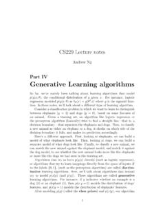
8 For example, data for the years IBM 1980-2006 might not lead to a good strategy for use in Dec. 2006. A more accurate policy would likely result from training with data from , p(t) ' ratiotraining iterationFigure 1. Training results for autoregressive random process. 1000 T, 75 eNThe first example of training a policy is executed on an autoregressive random process (randomness by injecting Gaussian noise into coupled equations). In figure 1, the top graph is the generated price series. The bottom graph is Sharpe s ratio on the time series using the parameterwfor each iteration of training. So, as training progresses, we find better values of w until we have achieved an optimum Sharpe s ratio for the given , we use this optimalw parameter to form a prediction for the next predictN data samples, shown below:Figure 2.

9 Prediction performance using optimal policy from training. 1000 predictNAs is apparent from the above graph, the trader is making decisions based on thewparameter. Of course, w is suboptimal for the time series over this predicted interval, but it does better than a monkey. After 1000 intervals our return would be 10%.The next experiment, presented in the same format, is to predict real Stock data with some precipitous drops(Citigroup):1002003004005006004060p rice series, 's ratiotraining iterationFigure 3. Trainingwon Citigroup Stock data. 600 T, 100 eN5600650700750800850900-15-10-505tretur ns, (decisions)t6006507007508008509000102030 tpercent gains (%)Figure 4. tr (top), tF (middle), and percentage profit (cumulative) for Citigroup.

10 Note that although the general policy is good, the precipitous drop in price (downward spike intr) wipes out our gains around t = 725. The Recurrent Reinforcement learner seems to work best on stocks that are constant on average, yet fluctuate up and down. In such a case, there is less worry about a precipitous drop like in the above example. With a relatively constant mean Stock price, the Reinforcement learner is free to play the ups and Recurrent Reinforcement learner seems to work, although it is tricky to set up and verify. One important trick is to properly scale the return series data to mean zero and variance one2, or the neuron cannot separate the resulting data CONCLUSIONSThe primary difficulties with this approach rest in the fact that certain Stock events do not exhibit structure.