Example: stock market
Lecture 13 Linear dynamical systems with inputs & outputs
Linear dynamical systems with inputs & outputs • inputs & outputs: interpretations • transfer matrix • impulse and step matrices • examples 13–1. Inputs & outputs recall continuous-time time-invariant LDS has form x˙ = Ax+Bu, y = Cx+Du • Ax is called the drift term (of x˙)
Tags:
Information
Domain:
Source:
Link to this page:
Documents from same domain

Lecture 3 Linear Equations and Matrices
see.stanford.eduso multiplication by matrix inverse solves a set of linear equations some comments: • x = A−1b makes solving set of 100 linear equations in 100 variables look simple, but the notation is hiding alot of work!

CS229 Lecture notes - Stanford Engineering Everywhere
see.stanford.eduwe decide to approximate y as a linear function of x: hθ(x) = θ0 +θ1x1 +θ2x2 Here, the θi’s are the parameters (also called weights) parameterizing the space of linear functions mapping from X to Y. When there is no risk of confusion, we will drop the θ …
EE364a Homework 3 solutions
see.stanford.eduEE364a Homework 3 solutions 3.42 Approximation width. Let f0,...,fn: R → R be given continuous functions. We ... Use part (c) to verify that f ... 4.8 Some simple LPs. Give an explicit solution of each of the following LPs. (a) Minimizing a linear function over an affine set. minimize cTx subject to Ax = b.

Lecture 15 Symmetric matrices, quadratic forms, matrix ...
see.stanford.edu• rotate by QT • diagonal real scale (‘dilation’) by Λ • rotate back by Q decomposition A = Xn i=1 λiqiq T i expresses A as linear combination of 1-dimensional projections Symmetric matrices, quadratic forms, matrix norm, and SVD 15–5
Probability Theory Review for Machine Learning
see.stanford.eduProbability Theory Review for Machine Learning Samuel Ieong November 6, 2006 1 Basic Concepts Broadly speaking, probability theory is the mathematical study of uncertainty.
Much of this handout was written by Justin Manus and ...
see.stanford.eduDownloading Eclipse Much of this handout was written by Justin Manus and Brandon Burr. This quarter we’ll be using Stanford’s customized version of Eclipse to build our programs. Eclipse is an enormously popular industrial strength Java environment with many, many features. Fortunately, Eclipse is also open source—anyone is free to change

cvx Users’ Guide - Stanford Engineering Everywhere
see.stanford.edu1.2 What is disciplined convex programming? Disciplined convex programming is a methodology for constructing convex optimiza-tion problems proposed by Michael Grant, Stephen Boyd, and …

CS 229, Public Course Problem Set #1 Solutions: Supervised ...
see.stanford.edu2. Locally-weighted logistic regression In this problem you will implement a locally-weighted version of logistic regression, where we weight different training examples differently according to the query point. The locally-weighted logistic regression problem is to maximize ℓ(θ) = − λ 2 θTθ + Xm i=1 w(i) h y(i) logh θ(x (i))+(1−y ...
Lecture 5 Least-squares - Stanford Engineering Everywhere
see.stanford.eduLeast-squares (approximate) solution • assume A is full rank, skinny • to find xls, we’ll minimize norm of residual squared, krk2 = xTATAx−2yTAx+yTy • set gradient w.r.t. x to zero: ∇xkrk2 = 2ATAx−2ATy = 0 • yields the normal equations: ATAx = ATy • assumptions imply ATA invertible, so we have xls = (ATA)−1ATy. . . a very famous formula
Convex Optimization — Boyd & Vandenberghe 3. Convex …
see.stanford.edu2. for twice differentiable functions, show ∇2f(x) 0 3. show that f is obtained from simple convex functions by operations that preserve convexity • nonnegative weighted sum • composition with affine function • pointwise maximum and supremum • composition • minimization • perspective Convex functions 3–13
Related documents

Algebra 1B Worksheet: Systems of Linear Inequalities
www.ozarktigers.orgAlgebra 1B Worksheet: Systems of Linear Inequalities Name: _____ Graph the following systems on linear inequalities 4. 5. Name 3 solutions to each of the following systems of linear inequalities 6. 7.
Solving Systems of Linear Inequalities
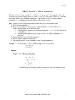
www.alamo.eduSolving Systems of Linear Inequalities . Solving a system of linear inequalities is similar to solving system of linear equations but with inequalities we are not finding a point (or points) of intersect. Instead the solution set will be the region that satisfies all of the linear inequalities. The best way to solve a system of linear
The Phase Plane Phase Portraits of Linear Systems
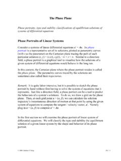
www.personal.psu.edusystems of differential equations Phase Portraits of Linear Systems Consider a systems of linear differential equations x′ = Ax. Its phase portrait is a representative set of its solutions, plotted as parametric curves (with t as the parameter) on the Cartesian plane tracing the path of each particular solution (x, y) = (x 1(t), x

6.4.9 Solutions to homogeneous systems of linear equations
ece.uwaterloo.casystems of linear equations Introduction • In this topic, we will –Review the definition of a homogenous system of linear equations –Compare solutions to non-homogenous and corresponding homogenous systems of linear equations –See that the zero vector is always a solution to a homogenous

Problem set 5: Properties of linear, time-invariant systems
ocw.mit.eduSignals and Systems P5-2 P5.4 Consider the linear, time-invariant system in Figure P5.4, which is composed of a cascade of two LTI systems. u(t) is a unit step signal and s(t) is the step response of system L. s(t) u(t) - L d/dt y(t) Figure P5.4 Using the fact that the overall response of LTI systems in cascade is indepen

Describing Solution Sets to Linear Systems
people.math.umass.eduHomogeneous Linear Systems: Ax = 0 Solution Sets of Inhomogeneous Systems Another Perspective on Lines and Planes Particular Solutions A Remark on Particular Solutions Observe that taking t = 0, we nd that p itself is a solution of the system: Ap = b. This is but one element in the solution set, and

Systems of Linear Equations - Department of Mathematics
math.colorado.eduSystems of Linear Equations 0.1 De nitions Recall that if A2Rm n and B2Rm p, then the augmented matrix [AjB] 2Rm n+p is the matrix [AB], that is the matrix whose rst ncolumns are the columns of A, and whose last p columns are the columns of B. Typically we consider B= 2Rm 1 ’Rm, a column vector.
Linear Systems: REDUCED ROW ECHELON FORM
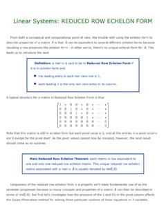
web.ma.utexas.eduLinear Systems: REDUCED ROW ECHELON FORM From both a conceptual and computational point of view, the trouble with using the echelon form to describe properties of a matrix is that can be equivalent to several different echelon forms because rescaling a row preserves the echelon form - in other words, there's no unique echelon form for . This

Systems of Two Equations - cdn.kutasoftware.com
cdn.kutasoftware.comSystems of Two Equations Author: Mike Created Date: 7/26/2012 1:50:05 PM ...