Transcription of Lecture 2: Geometric Image Transformations
1 Lecture 2: Geometric Image TransformationsHarvey RhodyChester F. Carlson Center for Imaging ScienceRochester institute of 8, 2005 AbstractGeometric Transformations are widely used for Image registrationand the removal of Geometric distortion. Common applications includeconstruction of mosaics, geographical mapping, stereo and Lecture 2 Spatial Transformations of ImagesA spatial transformation of an Image is a Geometric transformation of theimage coordinate is often necessary to perform a spatial transformation to: Align images that were taken at different times or with different sensors Correct images for lens distortion Correct effects of camera orientation Image morphing or other special effectsDIP Lecture 21 Spatial TransformationIn a spatial transformation each point(x, y)of imageAis mapped to apoint(u, v)in a new coordinate (x, y)v=f2(x, y)Mapping from(x, y)to(u, v)coordinates.
2 A digital Image array has an implicit gridthat is mapped to discrete points in the new domain. These points may not fall on gridpoints in the new Lecture 22 Affine TransformationAn affine transformation is any transformation that preserves collinearity( , all points lying on a line initially still lie on a line after transformation)and ratios of distances ( , the midpoint of a line segment remains themidpoint after transformation).In general, an affine transformation is a composition of rotations,translations, magnifications, and +c12y+c13v=c21x+c22y+c23c13andc23affect translations,c11andc22affect magnifications, and thecombination affects rotations and Lecture 23 Affine TransformationA shear in thexdirection is produced byu=x+ Lecture 24 Affine TransformationThis produces as both a shear and a + +yDIP Lecture 25 Affine TransformationA rotation is produced by is produced byu=xcos +ysin v= xsin +ycos DIP Lecture 26 Combinations of TransformsComplex affine transforms can be constructed by a sequence of basic combinations are most easily described in terms of matrixoperations.
3 To use matrix operations we introducehomogeneouscoordinates. These enable all affine operations to be expressed as amatrix multiplication. Otherwise, translation is an affine equations are expressed as uv1 = a b cd e f0 0 1 xy1 An equivalent expression using matrix notation isq=Tpwhereq,Tandqare the defined Lecture 27 Transform OperationsThe transformation matrices below can be used as building 1 0x00 1y00 0 1 Translation by(x0, y0)T= s10 00s200 0 1 Scale bys1ands2T= cos sin 0 sin cos 000 1 Rotate by You will usually want to translate the center of the Image to the origin ofthe coordinate system, do any rotations and scalings, and then translate Lecture 28 Combined Transform OperationsOperationExpressionResultTrans late toOriginT1= Rotate by 23degreesT2= Translate tooriginallocationT3= DIP Lecture 29 Composite Affine TransformationThe transformation matrix of a sequence of affine Transformations .
4 SayT1thenT2thenT3isT=T3T2T3 The composite transformation for the example above isT=T3T2T1= Any combination of affine Transformations formed in this way is an inverse transform isT 1=T 11T 12T 13If we find the transform in one direction, we can invert it to go the Lecture 210 Composite Affine Transformation RSTS uppose that you want the composite representation for translation, scalingand rotation (in that order).H=RST= cos sin 0 sin cos 000 1 s00 00s100 0 1 1 0x00 1x10 0 1 =[s0cos s1sin s0x0cos +s1x1sin s0sin s1cos s1x1cos s0x0sin ]Given the matrixHone can solve for the five Lecture 211 How to Find the TransformationSuppose that you are given a pair of images to align.
5 You want to try anaffine transform to register one to the coordinate system of the other. Howdo you find the transform parameters?ImageAImageBDIP Lecture 212 Point MatchingFind a number of points{p0,p1, .. ,pn 1}in imageAthat matchpoints{q0,q1, .. ,qn 1}in imageB. Use the homogeneous coordinaterepresentation of each point as a column in matricesPandQ:P= x0x1.. xn 1y0y1.. yn 11 1..1 =[p0p1..pn 1]Q= u0u1.. un 1v0v1.. vn 11 1..1 =[q0q1..qn 1]Thenq=HpbecomesQ=HPThe solution forHthat provides the minimum mean-squared error isH=QPT(PPT) 1=QP whereP =PT(PPT) 1is the (right) Lecture 213 Point MatchingThe transformation used in the previous example can be found from a fewmatching points chosen randomly in each Image processing tools, such as ENVI, have tools to enable point-and-click selection of matching Lecture 214 InterpolationInterpolation is needed to find the value of the Image at the grid points inthe target coordinate system.
6 The mappingTlocates the grid points ofAin the coordinate system ofB, but those grid points are not on the grid find the values on the grid points ofBwe need to interpolate from thevalues at the projected the closest projected points to a given grid point can becomputationally Lecture 215 Inverse ProjectionProjecting the grid ofBinto the coordinate system ofAmaintains the known Image valueson a regular grid. This makes it simple to find the nearest points for each the homogeneous grid coordinates ofBand letHbe the transformation fromAtoB. ThenP=H 1 Qgrepresents the projection fromBtoA. We want to find the value at each pointPgivenfrom the values onPg, the homogeneous grid coordinates Lecture 216 Methods of InterpolationThere are several common methods of interpolation: Nearest neighbor simplest and fastest Triangular Uses three points from a bounding triangle.
7 Useful evenwhen the known points are not on a regular grid. Bilinear Uses points from a bounding rectangle. Useful when the knownpoints are on a regular Lecture 217 Bilinear InterpolationSuppose that we want to find the valueg(q)at a pointqthat is interior to afour-sided figure with vertices{p0, p1, p2, p3}. Assume that these points arein order of progression around the figure and thatp0is the point farthestto the the point(xq, ya)betweenp0andp1. Computeg(xq, ya)by linearinterpolation betweenf(p0)andf(p1). the point(xq, yb)betweenp3andp2. Computeg(xq, yb)by linearinterpolation betweenf(p3)andf(p2). interpolate betweeng(xq, ya)andg(xq, yb)to findg(xq, yq).DIP Lecture 218 Triangular InterpolationLet(xi, yi, zi)i= 0,1,2be three pointsthat are not collinear.
8 These points forma triangle. Let(xq, yq)be a point insidethe triangle. We want to compute a valuezqsuch that(xq, yq, zq)falls on a planethat contains(xi, yi, zi),i= 0,1, interpolation will work even ifqisnot within the triangle, but, for accuracy,we want to use a bounding plane is described by an equationz=a0+a1x+a2yThe coefficients must satisfy the three equations that correspond to thecorners of the Lecture 219 Triangular Interpolation z0z1z2 = 1x0y01x1y11x2y2 a0a1a2 In matrix notation we can writez=Caso thata=C 1zThe matrixCis nonsingular as long as the triangle corners do not fall alonga line. Then the valuezqis given byzq=[1xqyq]a=[1xqyq]C 1zSinceCdepends only upon the locations of the triangle corners,(xi, yi),i= 0,1,2it can be computed once the triangles are known.
9 This is usefulin processing large batches of Lecture 220 Triangular Interpolation CoefficientsAfter some algebra we find the following equation for the coefficients neededto +c1z1+c2z2c0=x2y1 x1y2+xq(y2 y1) yq(x2 x1)(x1 x2)y0+ (x2 x0)y1+ (x0 x1)y2c1=x0y2 x2y0+xq(y0 y2) yq(x0 x2)(x1 x2)y0+ (x2 x0)y1+ (x0 x1)y2c2=x1y0 x0y1+xq(y1 y0) yq(x1 x0)(x1 x2)y0+ (x2 x0)y1+ (x0 x1)y2 Some simple algebra shows thatc0+c1+c2= 1 This is a useful computational check. It also enables the interpolationcalculation to be done with 33% less Lecture 221 Image MappingAtoBIf the projection fromBtoAis known then we the coordinates of theBpixels onto theApixel the nearestAgrid points for each projectedBgrid the value for theBpixels by interpolation of that there is no projection back toB.
10 We have computed the valuesfor we know that the coordinates ofAare integers then we can find the fourpixels ofAthat surround(xq, yq)by quantizing the coordinate Lecture 222 Image Mapping ExampleTwo images of the same scene with seven selected matching points areshown Lecture 223 Affine TransformThe matching points have coordinates shown in the first four columns of thetable below. From this we can form the homogeneous coordinate matricesPandQ. The mappingHfromAtoBisH=QP = The projection of the(Xa, Ya)points byHis shown in the lasttwo columns. These are close to the matching(Xb, Yb) of Matching PointsXaYaXbYbX aY Lecture 224 Image TransformationThe transformedAimage is on the right and the originalBimage is on theleft.