Transcription of Lecture 5 Least-squares - Stanford Engineering Everywhere
1 EE263 Autumn 2007-08 Stephen BoydLecture 5 Least-squares Least-squares (approximate) solution of overdetermined equations projection and orthogonality principle Least-squares estimation BLUE property5 1 Overdetermined linear equationsconsidery=AxwhereA Rm nis (strictly) skinny, ,m > n calledoverdeterminedset of linear equations(more equations than unknowns) for mosty, cannot solve forxone approach toapproximatelysolvey=Ax: defineresidualor errorr=Ax y findx=xlsthat minimizeskrkxlscalledleast-squares(appro ximate) solution ofy=AxLeast-squares5 2 Geometric interpretationAxlsis point inR(A)closest toy(AxlsisprojectionofyontoR(A))R(A)yAxl srLeast-squares5 3 Least-squares (approximate) solution assumeAis full rank, skinny to findxls, we ll minimize norm of residual squared,krk2=xTATAx 2yTAx+yTy set gradient zero: xkrk2= 2 ATAx 2 ATy= 0 yields thenormal equations:ATAx=ATy assumptions implyATAinvertible, so we havexls= (ATA) 1 ATy.
2 A very famous formulaLeast-squares5 4 xlsis linear function ofy xls=A 1yifAis square xlssolvesy=Axlsify R(A) A = (ATA) 1 ATis called thepseudo-inverseofA A is aleft inverseof (full rank, skinny)A:A A= (ATA) 1 ATA=ILeast-squares5 5 projection onR(A)Axlsis (by definition) the point inR(A)that is closest toy, , it is theprojectionofyontoR(A)Axls=PR(A)(y) the projection functionPR(A)is linear, and given byPR(A)(y) =Axls=A(ATA) 1 ATy A(ATA) 1 ATis called theprojection matrix(associated withR(A))Least-squares5 6 Orthogonality principleoptimal residualr=Axls y= (A(ATA) 1AT I)yis orthogonal toR(A).
3 Hr, Azi=yT(A(ATA) 1AT I)TAz= 0for allz RnR(A)yAxlsrLeast-squares5 7 Least-squares viaQRfactorization A Rm nskinny, full rank factor asA=QRwithQTQ=In,R Rn nupper triangular,invertible pseudo-inverse is(ATA) 1AT= (RTQTQR) 1 RTQT=R 1 QTsoxls=R 1 QTy projection onR(A)given by matrixA(ATA) 1AT=AR 1QT=QQTL east-squares5 8 Least-squares via fullQRfactorization fullQRfactorization:A= [Q1Q2] R10 with[Q1Q2] Rm morthogonal,R1 Rn nupper triangular,invertible multiplication by orthogonal matrix doesn t change norm, sokAx yk2= [Q1Q2] R10 x y 2= [Q1Q2]T[Q1Q2] R10 x [Q1Q2]Ty 2 Least-squares5 9= R1x QT1y QT2y 2=kR1x QT1yk2+kQT2yk2 this is evidently minimized by choicexls=R 11QT1y(which make first term zero) residual with optimalxisAxls y= Q2QT2y Q1QT1gives projection ontoR(A) Q2QT2gives projection ontoR(A)
4 Least-squares5 10 Least-squares estimationmany applications in inversion, estimation, and reconstructionproblemshave formy=Ax+v xis what we want to estimate or reconstruct yis our sensor measurement(s) vis an unknownnoiseormeasurement error(assumed small) ith row ofAcharacterizesith sensorLeast-squares5 11least-squares estimation: choose as estimate xthat minimizeskA x , deviation between what we actually observed (y), and what we would observe ifx= x, and there were no noise (v= 0) Least-squares estimate is just x= (ATA) 1 ATyLeast-squares5 12 BLUE propertylinear measurement with noise:y=Ax+vwithAfull rank, skinnyconsider alinear estimatorof form x=By calledunbiasedif x=xwheneverv= 0( , no estimation error when there is no noise)same asBA=I, ,Bis left inverse ofALeast-squares5 13 estimation error of unbiased linear estimator isx x=x B(Ax+v) = Bvobviously, then, we d likeB small (andBA=I) fact.
5 A = (ATA) 1 ATis thesmallestleft inverse ofA, in thefollowing sense:for anyBwithBA=I, we haveXi,jB2ij Xi,jA , Least-squares provides thebest linear unbiased estimator(BLUE)Least-squares5 14 Navigation from range measurementsnavigation using range measurements fromdistantbeaconsxk1k2k3k4beaconsunknow n positionbeacons far from unknown positionx R2, so linearization aroundx= 0(say) nearly exactLeast-squares5 15rangesy R4measured, with measurement noisev:y= kT1kT2kT3kT4 x+vwherekiis unit vector from0to beaconimeasurement errors are independent, Gaussian, with standard deviation2(details not important)problem:estimatex R2, giveny R4(roughly speaking, a2:1measurement redundancy ratio)actual position isx= ( , ).
6 Measurement isy= ( , , , )Least-squares5 16 Just enough measurements methody1andy2suffice to findx(whenv= 0)compute estimate xby inverting top (2 2) half ofA: x=Bjey= 0 0 0 0 0 y= (norm of )Least-squares5 17 Least-squares methodcompute estimate xby Least-squares : x=A y= y= (norm of ) BjeandA are both left inverses ofA larger entries inBlead to larger estimation errorLeast-squares5 18 Example from overview lectureuwyH(s)A/D signaluis piecewise constant, period1 sec,0 t 10:u(t) =xj, j 1 t < j, j= 1, .. ,10 filtered by system with impulse responseh(t):w(t) =Zt0h(t )u( )d sample at10Hz: yi=w( ),i= 1.
7 ,100 Least-squares5 19 3-bit quantization:yi=Q( yi),i= 1, .. ,100, whereQis 3-bitquantizer characteristicQ(a) = (1/4) (round(4a+ 1/2) 1/2) problem:estimatex R10giveny R100 101012345678910 101012345678910 101s(t)u(t)w(t)y(t)tLeast-squares5 20we havey=Ax+v, where A R100 10is given byAij=Zjj 1h( )d v R100isquantization error:vi=Q( yi) yi(so|vi| ) Least-squares estimate:xls= (ATA) 1 ATy012345678910 1 (t)(solid) & u(t)(dotted)tLeast-squares5 21 RMS error iskx xlsk 10= if we had no filtering! (RMS )more on this later ..Least-squares5 22some rows ofBls= (ATA) 1AT:012345678910 rows show how sampled measurements ofyare used to form estimateofxifori= 2,5,8 to estimatex5, which is the original input signal for4 t <5, wemostly usey(t)for3 t 7 Least-squares5 23