Transcription of LECTURE NOTES #6: Correlation and Regression
1 LECTURE NOTES #6: Correlation and Regression6-1 Richard GonzalezPsych 613 Version (Nov 2021) LECTURE NOTES #6: Correlation and RegressionReading assignment: Stay current with the readingKNNL Chapters 1, 2, 3, 4, and 15; CCWA chapters 1 and 2 There are several ways to think about Regression , and we will cover a few of them. Each perspective,or way of thinking about Regression , lends itself to answering different research questions. Usingdifferent perspectives on Regression will show us the generality of the technique, which will help ussolve new types of data analysis problems that we may encounter in our Describing bivariate bivariate normal distribution generalizes the normal distribution. See Figure 6-1 we want to find the relationship 1, or association, between two variables. Thiscan be done visually with a scatter plot. Examples of scatter plots are given in Figures 6-2and 6-3 with n=20 and n=500, Correlation is a quantitative measure to assess the linear association between two vari-ables.
2 The Correlation can be thought of as having two parts: one part that measures theassociation between variables and another part that acts like a normalizing constant. Thefirst part is called the covariance. To understand better the concept of covariance recall thedefinition of sums of squaresSY=X(Y Y)2(6-1)=X(Y Y)(Y Y)(6-2)This is the sum of the product of the differences between the scores and the mean. Theestimated variance of Y isSYN 1(6-3)1 Some people quibble about whether to refer to a Correlation between two variables as a relation or a relationship .I suppose proper usage would have a relation refer to two variables and a relationship refer to the bond between twopeople. But I m not bothered such things and tend to use NOTES #6: Correlation and Regression6-2 Figure 6-1: Bivariate Density Function-4-2 024X-4-2 024Y ; s1=s2=1; rho= $ $ ; s1=s2=1; rho=0-4-2 024X-4-2 024Y ; s1=s2=1; rho= $ $ ; s1=s2=1; rho= 024X-4-2 024Y ; s1=s2=1; rho= $ $ ; s1=s2=1; rho= NOTES #6: Correlation and Regression6-3 Figure 6-2: Varying : Each scatter plot contains a sample with 20 points.
3 Xy-2-101-3-2-10123mu1=mu2=0; s1=s2=1; rho=0 xy-2-101-3-2-10123mu1=mu2=0; s1=s2=1; rho= ; s1=s2=1; rho= ; s1=s2=1; rho= ; s1=s2=1; rho= xy-1012-3-2-10123mu1=mu2=0; s1=s2=1; rho= xy-1012-3-2-10123mu1=mu2=0; s1=s2=1; rho= xy-2-101-3-2-10123mu1=mu2=0; s1=s2=1; rho= NOTES #6: Correlation and Regression6-4 Figure 6-3: Varying : Each scatter plot contains a sample with 500 points. xy-3-2-10123-3-2-10123mu1=mu2=0; s1=s2=1.
4 Rho=0 xy-3-2-1012-3-2-10123mu1=mu2=0; s1=s2=1; rho= xy-3-2-10123-3-2-10123mu1=mu2=0; s1=s2=1.
5 Rho= xy-3-2-10123-3-2-10123mu1=mu2=0; s1=s2=1; rho= xy-2-10123-3-2-10123mu1=mu2=0; s1=s2=1.
6 Rho= xy-3-2-10123-3-2-10123mu1=mu2=0; s1=s2=1; rho= xy-3-2-1012-3-2-10123mu1=mu2=0; s1=s2=1.
7 Rho= xy-202-3-2-10123mu1=mu2=0; s1=s2=1; rho= NOTES #6: Correlation and Regression6-5 The covariance is similar to the variance except that it is defined over two variables (X andY) rather than one (Y). We begin with the numerator of the covariance it is the sums ofsquares of the two (X X)(Y Y)(6-4)The (estimated) covariance isSxyN 1(6-5)The interpretation of the covariance is similar to that of the variance. The covariance is ameasure of both the direction and the magnitude of the linear association between X and will a covariance be positive?
8 Negative?The covariance can be viewed intuitively as a sum of matches in terms of a subject beingon the same side of the mean on each variable. That is, for a particular subject a match wouldmean that the subject is, say, greater than the mean on variable Xandis also greater thanthe mean on variable Y. A mismatch is defined for a subject as the score on variable X isgreater than the mean but the score on variable Y is less than the mean, or vice versa. For aparticular subject i, a match leads to a positive product in Equation 6-4 whereas a mismatchleads to a negative can think of the variance as the covariance of a variable with itself, denoted Sxx/(N 1).InthesenotesSxx=SxThe covariance of a variable with itself and the variance of that variable are identical. I willuse Sxx/(N 1)and Sx/(N 1)interchangeably to denote the variance of covariance has the property that adding a constant to either variable does not change thecovariance, ,S(x+c)yN 1=SxyN 1(6-6)and multiplying either variable by a constant changes the covariance by a multiple of thatconstant, ,cSxyN 1=S(cx)yN 1(6-7)The property that multiplying by a constant changes the covariance can make interpreting thecovariance difficult because we would get a different covariance if we used one measurementas opposed to another ( , length in feet v.)
9 Length in yards). One simple trick fixes thisscaling problem. Recall that the standard deviation also has these two properties (adding aconstant doesn t change the standard deviation and multiplying by a constant changes theLecture NOTES #6: Correlation and Regression6-6standard deviation by a multiple of that constant). So, the standard deviations can be used to normalize the covariance such thatdefinition:correlationcovariance(X,Y ) (X) (Y)(6-8)SxyqSxSy(6-9)Dividing by the standard deviation makes the scaling constant c cancel out. The N - 1 termsin both the numerator and denominator of Equation 6-8 also cancel. Thus, Equation 6-9 canbe interpreted as a ratio of sums of squares, equivalently as the ratio of the covariance tothe product of the standard have just defined a useful concept. Equation 6-8 is the definition of thecorrelation coef-ficient(and so is Equation 6-9). The Correlation is the covariance normalized by the standarddeviations of the two variables and ranges from -1 to 1.
10 The normalization removes the scal-ing issue mentioned in the previous paragraph about multiplying by a constant. The samplecorrelation is denoted rxy(sometimes just r for short).3 The Correlation squared, denoted r2xy, has an interesting interpretation: it is the proportionof the variability in one variable that can be accounted for bya linear functionof the othervariable. It turns out that Regression has a structural model that is analogous to the structuralmodel we saw for ANOVA. The structural model for the Correlation is Y = 0+ 1X + ,where 0is the intercept (analogous to the grand mean ). 1is the slope (analogous to thetreatment effect in ANOVA), and is the usual error we know that proportions add up to 100%, if the r2xyis the proportion of variancethat is explained, then (1-r2xy) is the proportion of the variance that is not explained. That is,r2xy+ (1 r2xy) = 1(6-10)We will discuss what is meant by variance accounted for later, but for now we can makeuse of concepts from ANOVA.