Transcription of LECTURE NOTES - VI
1 LECTURE NOTES - VI fluid mechanics Prof. Dr. At l BULU Istanbul Technical University College of Civil Engineering Civil Engineering Department Hydraulics Division CHAPTER 6 TWO- dimensional IDEAL FLOW INTRODUCTION An ideal fluid is purely hypothetical fluid , which is assumed to have no viscosity and no compressibility, also, in the case of liquids, no surface tension and vaporization. The study of flow of such a fluid stems from the eighteenth century hydrodynamics developed by mathematicians, who, by making the above assumptions regarding the fluid , aimed at establishing mathematical models for fluid flows. Although the assumptions of ideal flow appear to be far obtained, the introduction of the boundary layer concept by Prandtl in 1904 enabled the distinction to be made between two regimes of flow: that adjacent to the solid boundary, in which viscosity effects are predominant and, therefore, the ideal flow treatment would be erroneous, and that outside the boundary layer, in which viscosity has negligible effect so that idealized flow conditions may be applied.
2 The ideal flow theory may also be extended to situations in which fluid viscosity is very small and velocities are high, since they correspond to very high values of Reynolds number, at which flows are independent of viscosity. Thus, it is possible to see ideal flow as that corresponding to an infinitely large Reynolds number and zero viscosity. CONTINUITY EQUATION The control volume ABCDEFGH in Fig. is taken in the form of a small prism with sides dx, dy and dz in the x, y and z directions, respectively. zxyBADEHCG dxdzdy Fig. The mean values of the component velocities in these directions are u, v, and w. Considering flow in the x direction, Mass inflow through ABCD in unit time udydz = Prof.
3 Dr. At l BULU 100In the general case, both specific mass and velocity u will change in the x direction and so, Mass outflow through EFGH in unit time ()dydzdxxuu += Thus, Net outflow in unit time in x direction ()dxdydzxu = Similarly, Net outflow in unit time in y direction ()dxdydzyv = Net outflow in unit time in z direction ()dxdydzzw = Therefore, Total net outflow in unit time ()()()dxdydzzwyvxu + + = Also, since / t is the change in specific mass per unit time, Change of mass in control volume in unit time dxdydzt = (the negative sign indicating that a net outflow has been assumed). Then, Total net outflow in unit time = Change of mass in control volume in unit time ()()()dxdydztdxdydzzwyvxu = + + or ()()()tzwyvxu = + + ( ) Equ.
4 ( ) holds for every point in a fluid flow whether steady or unsteady, compressible or incompressible. However, for incompressible flow, the specific mass is constant and the equation simplifies to 0= + + zwyvxu ( ) For two- dimensional incompressible flow this will simplify still further to 0= + yvxu ( ) Prof. Dr. At l BULU 101 EXAMPLE : The velocity distribution for the flow of an incompressible fluid is given by u = 3-x, v = 4+2y, w = 2-z. Show that this satisfies the requirements of the continuity equation. SOLUTION: For three- dimensional flow of an incompressible fluid , the continuity equation simplifies to Equ.
5 ( ); 1,2,1 = = = zwyvxu and, hence, 0121= + = + + zwyvxu Which satisfies the requirement for continuity. EULER S EQUATIONS Euler s equations for a vertical two- dimensional flow field may be derived by applying Newton s second law to a basic differential system of fluid of dimension dx by dz (Fig. ). dFzdWdxdFxxzazuzdzaxuxgCDBA Fig. The forces dFx and dFz on such an elemental system are, gdxdzdxdzzpdFdxdzxpdFzx = = The accelerations of the system have been derived for steady flow (Equ. ) as, Prof. Dr. At l BULU 102zwwxwuazuwxuuazx + = + = Applying Newton s second law by equating the differential forces to the products of the mass of the system and respective accelerations gives, + = + = zwwxwudxdzgdxdzdxdzzpzuwxuudxdzdxdzxp and by cancellation of dxdz and slight arrangement, the Euler equations of two- dimensional flow in a vertical plane are zuwxuuxp + = 1 ( ) gzwwxwuzp+ + = 1 ( ) Accompanied by the equation continuity, 0= + zwxu ( )
6 The Euler equations form a set of three simultaneous partial differential equations that are basic to the solution of two- dimensional flow field problems; complete solution of these equations yields p, u and w as functions of x and z, allowing prediction of pressure and velocity at any point in the flow field. BERNOULLI S EQUATION Bernoulli s equation may be derived by integrating the Euler equations for a constant specific weight flow. Multiplying Equ. ( ) by dx and Equ. ( ) by dz and integrating from 1 to 2 on a streamline give = + = + 2121212121212111dzgdzzpdzzwwdzxwudxxpdxz uwdxxuu Prof. Dr. At l BULU 103uwV12xzdzudxdsVw However, along a streamline in any steady flow dz/dx=w/u and therefore udz = wdx.
7 If we collect the both equations, + = + + + 212121211dzgdzzpdxxpdzzwwzuudxxwwxuu Since ()xuxuu = 22, arranging the equation yields, ()()()() + = + + + 21212122212212222dzgdzzpdxxpdzzwdxxwdzzu dxxu Since the terms in each bracket is a total differential, by integrating gives ()(12122122212212222zzgppwwuu = + ) By remembering that V2 = u2 + w2, the equation takes the form of 2222112122zpgVzpgV++=++ ( ) This equation is the well-known Bernoulli equation and valid on the streamline between points 1 and 2 in a flow field. ROTATIONAL AND IRROTATIONAL FLOW Considerations of ideal flow lead to yet another flow classification, namely the distinction between rotational and irrotational flow.
8 Prof. Dr. At l BULU 104dydxd ( a )( b )( a )( b ) Fig. and Basically, there are two types of motion: translation and rotation. The two may exist independently or simultaneously, in which case they may be considered as one superimposed on the other. If a solid body is represented by square, then pure translation or pure rotation may be represented as shown in Fig. (a) and (b), respectively. If we now consider the square to represent a fluid element, it may be subjected to deformation. This can be either linear or angular, as shown in Fig. (a) and (b), respectively. The rotational movement can be specified in mathematical terms. shows the rotation of a rectangular fluid element in a two- dimensional flow.
9 X t xvv xvx 1uAB2 D' y tuyC'B'u yuyvxyx C Fig. During the time interval t the element ABCD has moved relative to A to a new position, which is indicated by the dotted lines. The angular velocity (wAB) of line AB is, Prof. Dr. At l BULU 105()xvtxtxxvtwttAB = = = limlim010 Similarly, the angular velocity (wAD) of line AD is yutwtAD = = 20lim The average of the angular velocities of these two line elements is defined as the rotation w of the fluid element ABCD. Therefore, () =+=yuxvwwwADAB2121 ( ) The condition of irrotationality for a two- dimensional flow is satisfied when the rotation w is everywhere zero, so that 0= yuxv or yuxv = ( ) For a three- dimensional flow, the condition of irrotationality requires that the rotation about each of three axes, which are parallel to x, y and z-axes must be zero.
10 Therefore, the following three equations must be satisfied: yuxvxwzuzvyw = = = ,, ( ) EXAMPLE : The velocity components in a two- dimensional velocity field for an incompressible fluid are expressed as 32233223xyxyvyxxyu = += Show that these functions represent a possible case of an irrotational flow. SOLUTION: The functions given satisfy the continuity equation (Equ. ), for their partial derivatives are xyxu22 = and 22 = xyyv so that 02222= + = + xyxyyvxu Prof. Dr. At l BULU 106 Therefore they represent a possible case of fluid flow. The rotation w of any fluid element in the flow field is, ()()[]0212332212122222332= = + = =xyxyyxxyyxyxyxyuxvw CIRCULATION AND VORTICITY Consider a fluid element ABCD in rotational motion.