Transcription of Maximum and Minimum Values - Pennsylvania State …
1 Multivariate Calculus; Fall 2013 S. Jamshidi Maximum and Minimum Values Objectives I can define critical points. I know the di erence between local and absolute minimums/maximums. I can find local Maximum (s), Minimum (s), and saddle points for a given function. I can find absolute Maximum (s) and Minimum (s) for a function over a closed set D. In many physical problems, we're interested in finding the Values (x, y) that maximize or mini- mize f (x, y). Recall from your first course in calculus that critical points are Values , x, at which the function's derivative is zero, f 0 (x) = 0. These x- Values either maximized f (x) (a Maximum ) or minimized f (x) (a Minimum ). We did not simply call a critical point a Maximum or a Minimum , however. Sometimes your critical point is local, meaning it's not the highest/lowest value achieved by the function, but it's the highest/lowest point near by.
2 See the image below for clarification. absolute Minimum local max local min absolute Maximum 135 of 155. Multivariate Calculus; Fall 2013 S. Jamshidi To classify critical points as maximums or minimums, we look at the second derivative. The point was called a Minimum if f 00 (x0 ) > 0 and it was called a Maximum if f 00 (x0 ) < 0. I like the mnemonic, concave up (+) is like a cup; concave down (-) is like a frown.. For functions of two variables, z = f (x, y), we do something similar. Definition A point (a, b) is a critical point of z = f (x, y) if the gradient, rf , is the zero vector. Critical points in three dimensions can be maximums, minimums, or saddle points. A saddle point mixes a Minimum in one direction with a Maximum in another direction, so it's neither (see the image below).
3 4. 2. 0. 2. 2. 4. 2 0. 1 0 1 2 2. Once a point is identified as a critical point, we want to be able to classify it as one of the three possibilities. Like you did in calculus, you will look at the second derivative. In higher dimensions, this is the determinant of a matrix containing all possible second derivatives. This matrix is called the Hessian matrix. f (a, b) fxy (a, b). det xx fyx (a, b) fyy (a, b). If you are not comfortable with matrices, you may may memorize the following formula d = fxx (a, b)fyy (a, b) [fxy (a, b)]2. 136 of 155. Multivariate Calculus; Fall 2013 S. Jamshidi The critical point is classified by the value of D. If d > 0 and fxx (a, b) > 0, then the point is a (local) Minimum . For fxx we can think, concave up (+) is like a cup.
4 If d > 0 and fxx (a, b) < 0, then the point is a (local) Maximum . For fxx we can think, concave down (-) is like a frown.. If d < 0, then the point is a saddle point. If d = 0, then the test fails and the point could be anything. Examples Example Find and classify all critical Values for the following function. f (x, y) = xy 2x 2y x2 y2. First, we need to find the zeros of the partial derivatives. Those partials are fx (x, y) = y 2 2x fy (x, y) = x 2 2y Set both of these partial derivatives to zero. 0=y 2 2x 0=x 2 2y Then we solve the system of equations. x = 2 + 2y =) y = 2 + 2(2 + 2y) =) y = 2 + 4 + 4y Then 3y = 6 gives us that y = 2. We can plug in to find x x = 2 + 2( 2) = 2. The solution is ( 2, 2). That is our critical point. Now, we need to classify it.
5 Let's find the second partial derivatives: 137 of 155. Multivariate Calculus; Fall 2013 S. Jamshidi fxx (x, y) = 2. fyy (x, y) = 2. fxy (x, y) = 1. Then d = ( 2)( 2) 1=3. Since d = 3 > 0 and fxx = 2 < 0, then we have a local Maximum . Example Find and classify all critical Values for the following function. f (x, y) = x3 12xy 8y 3. First, we need to find the zeros of the partial derivatives. Those partials are fx (x, y) = 3x2 12y fy (x, y) = 12x 24y 2. Set both of these partial derivatives to zero. y = (1/4)x2. x= 2y 2. Next, we solve the system of equations. y = (1/4)( 2y 2 )2 =) y = y 4. If y = 1, then x = 2. If y = 0, then x = 0. The critical points ( 2, 1) and (0, 0). We now calculate the second derivatives to classify the critical point.
6 Fxx (x, y) = 6x fyy (x, y) = 48y fxy (x, y) = 12. 138 of 155. Multivariate Calculus; Fall 2013 S. Jamshidi Then d = (6x)( 48y) (12)2 = 288xy 144. Now, let's determine d for the point ( 2, 1). d( 2, 1) = 576 144 = 432 > 0. Since d( 2, 1) = 432 > 0 and fxx ( 2, 1) = 6( 2) = 12 < 0, then ( 2, 1) a local Maximum . d(0, 0) = 0 144 < 0. Thus, (0, 0) is a saddle point. Example Find and classify all critical Values for the following function. f (x, y) = y cos(x). As before, we begin by finding the partial derivatives: fx (x, y) = y sin(x). fy (x, y) = cos(x). Set both of these equations equal to zero. 0= y sin(x). 0 = cos(x). For these equations to hold, we have the following conditions: y = 0, or x = , 0, , . x = 3 /2, /2, /2, 3 /2, . The only way to make both partial derivatives zero is to choose x = 3 /2, /2, /2, 3 /2.
7 Y=0. Therefore, the critical Values are ( 3 /2, 0), ( /2, 0), ( /2, 0), (3 /2, 0) . Now, we want to classify these points. To do that, we will calculate d. 139 of 155. Multivariate Calculus; Fall 2013 S. Jamshidi fxx (x, y) = y cos(x). fxy (x, y) = sin(x). fyy (x, y) = 0. Then d=0 sin2 (x) 0. For the points, ( 3 /2, 0), ( /2, 0), ( /2, 0), (3 /2, 0) . d is never zero. Therefore, d < 0 and that means all these critical points are saddles. If the domain is a closed set, then f has an absolute Minimum and an absolute Maximum . A closed set is a set that includes its boundary points. For example D1 = {(x, y)|x2 + y 2 2}. is closed because it includes its boundary while D2 = {(x, y)|x2 + y 2 < 2} is not closed because it does not. D1 D2. To find the absolute Maximum and absolute Minimum , follow these steps: 1.
8 Find the the critical points of f on D. 2. Find the extreme Values of f on the boundary of D. 3. The largest of the Values from steps 1 and 2 is the absolute Maximum value ; the smallest of these Values is the absolute Minimum value . 140 of 155. Multivariate Calculus; Fall 2013 S. Jamshidi The most challenging part of these problems will be considering the Values of f on the boundary. You will reduce the problem in one of two ways. Let's consider the domain D1 above and try to maximize f (x, y) = xy on its boundary. One method is to solve one variable p in terms of another. The boundary is 2 = x2 + y 2 , so could solve and say y = 2 x2 . Then we can plug in for y to get f (x, y) = f (x) =. we p x 2 x2 . The boundary's critical points are precisely those Values of x for which 2(x2 1).
9 0 = f 0 (x) = p 2 x2. This is only true when x = 1. We then find the corresponding Values of y and find the extreme points on the boundary are (1, 1), (1, 1), ( 1, 1), and ( 1, 1). p Alternatively, p we could parameterize the boundary. That means we pick x = 2 sin t and y = 2 cos t. Then we get f (t) = x(t)y(t) = 2 sin t cos t = sin 2t. We find the critical points of f (t) by solving 0 = f 0 (t) = 2 cos 2t. Here, we need to consider all Values of t between 0 and 2 because that is a full rotation around the boundary. Therefore, p this p is true if t = /4, 3 /4, 5 /4, and 7 /4. That means our extreme points are ( 2 sin t, 2 cos t) for those Values of t. That is, (1, 1), (1, 1), ( 1, 1), and ( 1, 1). Either approach will work. I recommend you use the one that makes the most sense to you in the given problem.
10 Before we look at examples, let's briefly discuss terminology. When we say critical points, we mean points where the derivative or gradient equals zero (f 0 (x) = 0 or rf = ~0). We use the term extreme value to just mean the biggest or smallest. The distinction is that an extreme value may not make the derivative zero, but it still may give the largest value . Examples Example Find the absolute Maximum and Minimum Values of the function on D, where D is the enclosed triangular region with vertices (0, 0), (0, 2), and (4, 0). f (x, y) = x + y xy Let's first draw a picture of D to help us visualize everything. 141 of 155. Multivariate Calculus; Fall 2013 S. Jamshidi x y= +2. 2. x=0. y=0. First, we find the critical points on D. We begin by finding the partials and setting them equal to zero fx (x, y) = 1 y=0.