Mean and Standard Deviation - University of York

1 1 Health Sciences Programme Applied Biostatistics Mean and Standard Deviation The mean The median is not the only measure of central value for a distribution. Another is the arithmetic mean or average, usually referred to simply as the mean. This is found by taking the sum of the observations and dividing by their number. The mean is often denoted by a little bar over the symbol for the variable, x. The sample mean has much nicer mathematical properties than the median and is thus more useful for the comparison methods described later. The median is a very useful descriptive statistic, but not much used for other purposes. Median, mean and skewness The sum of the 57 FEV1s is and hence the mean is = This is very close to the median, , so the median is within 1% of the mean. This is not so for the triglyceride data.

2 The median triglyceride is but the mean is , which is higher. The median is 10% away from the mean. If the distribution is symmetrical the sample mean and median will be about the same, but in a skew distribution they will not. If the distribution is skew to the right, as for serum triglyceride, the mean will be greater, if it is skew to the left the median will be greater. This is because the values in the tails affect the mean but not the median. Figure 1 shows the positions of the mean and median on the histogram of triglyceride. We can see that increasing the skewness by making the observation above much bigger would have the effect of increasing the mean, but would not affect the median. Hence as we make the distribution more and more skew, we can make the mean as large as we like without changing the median.

3 This is the property which tends to make the mean bigger than the median in positively skew distributions, less than the median in negatively skew distributions, and equal to the median in symmetrical distributions. Variance The mean and median are measures of the central tendency or position of the middle of the distribution. We shall also need a measure of the spread, dispersion or variability of the distribution. The most commonly used measures of dispersion are the variance and Standard Deviation , which I will define below. We start by calculating the difference between each observation and the sample mean, called the deviations from the mean. Some of these will be positive, some negative. 2 Figure 1. Histogram of serum triglyceride in cord blood, showing the positions of the mean and median If the data are widely scattered, many of the observations will be far from the mean and so many deviations will be large.

4 If the data are narrowly scattered, very few observations will be far from the mean and so few deviations will be large. We need some kind of average Deviation to measure the scatter. If we add all the deviations together, we get zero, so there is no point in taking an average Deviation . Instead we square the deviations and then add them. This removes the effect of plus or minus sign; we are only measuring the size of the Deviation , not the direction. This gives us the sum of squares about the mean, usually abbreviated to sum of squares. In the FEV1 example the sum of squares is equal to Clearly, the sum of squares will depend on the number of observations as well as the scatter. We want to find some kind of average squared Deviation . This leads to a difficulty. Although we want an average squared Deviation , we divide the sum of squares by the number of observations minus one, not the number of observations.

5 This is not the obvious thing to do and puzzles many students of statistical methods. The reason is that we are interested in estimating the scatter of the population, rather than the sample, and the sum of squares about the sample mean is not proportional to the number of observations. This is because the mean which we subtract is also calculated from the same observations. If we have only one observation, the sum of squares must be zero. The sum of squares cannot be proportional to the number of observations. Dividing by the number of observations would lead to small samples producing lower estimates of variability than large samples from the same population. In fact, the sum of squares about the sample mean is proportional to the number of observations minus one. If we divide the sum of squares by the number of observations minus one, the measure of variability will not be related to the sample size.

6 The estimate of variability found in this way is called the variance. The quantity is called the degrees of freedom of the variance estimate, often abbreviated to df or DF. We shall come across this term several times. It derived from probability theory and we shall accept it as just a name . We often denote the variance calculated from a sample by s2. 3 For the FEV data, s2 = (57 1) = Variance is based on the squares of the observations. FEV1 is measured in litres, so the squared deviations are measured in square litres, whatever they are. We have for FEV1: variance = litres2. Similarly, gestational age is measured in weeks and so the gestational age: variance = weeks2. A square week is another quantity hard to visualise. Variance is based on the squares of the observations and so is in squared units.

7 This makes it difficult to interpret. For this reason we often use the Standard Deviation instead, described below. Standard Deviation The variance is calculated from the squares of the observations. This means that it is not in the same units as the observations, which limits its use as a descriptive statistic. The obvious answer to this is to take the square root , which will then have the same units as the observations and the mean. The square root of the variance is called the Standard Deviation , usually denoted by s. It is often abbreviated to SD. For the FEV data, the Standard Deviation = = litres. Figure 2 shows the relationship between mean, Standard Deviation and frequency distribution for FEV1. Because Standard Deviation is a measure of variability about the mean, this is shown as the mean plus or minus one or two Standard deviations.

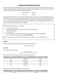
8 We see that the majority of observations are within one Standard Deviation of the mean, and nearly all within two Standard deviations of the mean. There is a small part of the histogram outside the mean plus or minus two Standard deviations interval, on either side of this symmetrical histogram. For the serum triglyceride data, s = = mmol/litre. Figure 3 shows the position of the mean and Standard Deviation for the highly skew triglyceride data. Again, we see that the majority of observations are within one Standard Deviation of the mean, and nearly all within two Standard deviations of the mean. Again, there is a small part of the histogram outside the mean plus or minus two Standard deviations interval. In this case, the outlying observations are all in one tail of the distribution, however.

9 For the gestational age data, s = = weeks. Figure 4 shows the position of the mean and Standard Deviation for this negatively skew distribution. Again, we see that the majority of observations are within one Standard Deviation of the mean, and nearly all within two Standard deviations of the mean. Again, there is a small part of the histogram outside the mean plus or minus two Standard deviations interval. In this case, the outlying observations are almost all in the lower tail of the distribution. In general, we expect roughly 2/3 of observations or more to lie within one Standard Deviation of the mean and about 95% to lie within two Standard deviations of the mean. 4 Figure 2. Histogram of FEV1 with mean and Standard Deviation marked. Figure 3. Histogram of serum triglyceride with positions of mean and Standard Deviation marked Figure 4.

10 Histogram of gestational age with mean and Standard Deviation marked. xx-sx-2sx+sx+2s0100200300400500 Frequency202530354045 Gestational age (weeks) +2sx+sx-sx-2sxFrequency2345605101520 FEV1 (litre)x+2sx+sxx-sx-2s5 Figure 5. Distribution of height in a sample of pregnant women, with the corresponding Normal distribution curve Spotting skewness Histograms are fairly unusual in published papers. Often only summary statistics such as mean and Standard Deviation or median and range are given. We can use these summary statistics to tell us something about the shape of the distribution. If the mean is less than two Standard deviations, then any observation less than two Standard deviations below the mean will be negative. For any variable which cannot be negative, this tells us that the distribution must be positively skew.