Transcription of mgcv: GAMs in R
1 Mgcv: GAMs in RSimon WoodMathematical Sciences, University of Bath, ,gamm4 mgcvis a package supplied with R for generalized additivemodelling, including generalized additive mixed models. The main GAM fitting routine isgam. bamprovides an alternative for very large datasets. The main GAMM fitting isgammwhich uses PQL based onpackagenlme. gamm4is an R package available , a version ofgammwhich useslme4forGAMM fitting, and avoids PQL. It is really an extensionpackage formgcv. The packages are loaded into R using (mgcv).mgcvhelp To get overview help ()within R andfollow thePackageslink tomgcv. The help pagemgcv-packageis a good page to start to getan overview.
2 Note other overview pages such All user visible functions are documented. Once a library is loaded its help pages are accessible via, ("gam")or?gam. Technical references on the underlying methods are given in?gamand viacitation("mgcv"). Wood (2006)Generalized additive models:an introductionwith RCRC/Taylor&Francis provides further Use of the functiongamis similar to the use of functionglm,except for the model formula can contain smooth termssand tensorproduct smooth termstein the linear are extra arguments controlling smoothing parameterestimation, notablymethodfor choosing between"REML","ML"," "and" "smoothness can also beTweedieornegbin.
3 Gamreturns and object of class"gam", which can be furtherinterrogated using method functions such asprint,summary,anova, plot ,predict,resid ualsetc. The front end design ofgamand its associated functions isbased heavily on Trevor Hastie s originalgamfunction underlying model representation and numerical methodsare very different, however, being based on the penalizedregression spline methods covered in this usable withgam gaussian(default) is useful for real valued response data. Gammais useful for strictly positive real valued data. The default link is onlyuseful in some waiting time applications, and the log link ismore often used.
4 Poissonis useful when the response is count data of some sort. binomialis used most often for binary (logistic) regression, but is applicable toany response that is the number of successes from a known number of trials. for strictly positive real response variables: useful forvarious time to event data. quasidoes not define a full distribution, but allows inference when only themean variance relationship can be well special cases. Not useable with likelihood based smoothnessselection. Tweedieis an alternative to quasi when var(y) = p, 1<p<2, and a fulldistribution is required (for a non-negative real response).
5 Negbinis useful for overdispersed count data, but computation is models: some examples yi=f(xi) + iwhere i N(0, 2)gam(y ~ s(x)) log{E(yi)}=f1(xi) +f2(zi) +f3(vi) +wiwhereyi (y ~ s(x) + s(z) + s(v) + w,family=poisson) E(yi) =f1(timei,distancei) +f2(wi),yi (y ~ te(time,distance) + s(w),family=Gamma(link=sqrt))uses a scale invariant tensor product smooth forf1. logit{E(yi)}=wif1(xi,zi) +f2(vi),yi (y ~ s(x,z,by=w) + s(v),family=binomial)Heref1is isotropic (a thin plate spline).sterm details s(x,k=20,id=2,bs="tp")is an example smooth specifier,used in a formula. (Some) arguments are ..xis the covariate of the smooth (can have any name!)
6 : sometypes of smooth can have several covariates ( tp ).bsis the type of basis-penalty the basis dimension for the smooth (before imposing anyidentifiability constraints).idused to allow different smooths to be forced to use the samebasis and smoothing the smoothing parameter to be the term is specification of interactions of the smooth with a factoror metric the penalty order for some classes Built in smooth classes ( options for thebsargument ofs)are:"cr"a penalized cubic regression spline ( cc for cyclic version)."ps"Eilers and Marx style P-splines ( cp for cyclic)."ad"adaptive smoothers based on ps.
7 "tp"Optimal low rank approximation to thin plate spline, anydimension and permissable penalty order is possible. In addition the"re"class implements simple random examples(x,z,bs="re")specifies a random effectZbwhereb N(0,I 2b).Zis given (~x:z-1).This approach is slow for large numbers od random effects,however. New classes can be added. See? product smoothing inmgcv Tensor product smooths are constructed automatically frommarginalsmooths of lower dimension. The resulting smoothhas a penalty for each marginal basis. mgcvcan construct tensor product smooths from anysinglepenaltysmooths useable withsterms.
8 Teterms within the model formula invoke this example: te(x,z,v,bs="ps",k=5)creates a tensor product smooth ofx, z and v using rank 5 P-spline marginals: the resultingsmooth has 3 penalties and basis dimension 125. te(x,z,t,bs=c("tp","cr"),d=c(2,1),k=(20, 5))createsa tensor product of an isotropic 2-D TPS with a 1-D smoothin time. The result is isotropic in x,z, has 2 penalties and abasis dimension of 100. This sort of smooth would beappropriate for a location-time data example To illustrate the basics ofgam, consider a very simple datasetrelating the timber volume of cherry trees to their height andtrunk 20 30 40 50 60 7010305070 Volumetreesinitialgamfit A possible model islog( i) =f1(Heighti)+f2(Girthi),Volumei Gamma( i, ) Using rank 10 thin plate regression splines as the smoothers.
9 Library(mgcv)ct1 <- gam(Volume ~ s(Height) + s(Girth),family=Gamma(link=log),data=trees)estimates the model with default GCV smoothness selection. The results are stored in class"gam"objectct1. For the full contents of a"gam"object see? Typingct1causes R to passct1to theprintmethodfunction. For class"gam"objectct1this means printing > ct1 Family: GammaLink function: logFormula:Volume ~ s(Height) + s(Girth)Estimated degrees of total = score: Notice how the EDFs for each term and the GCV score par(mfrow=c(1,2)) plot (ct1,residuals=TRUE ,pch=19) ## calls (Height,1)810 12 14 16 18 20 (Girth, ) partialresiduals forfjareweighted working residualsfrom PIRLS added to departure fromfjindicates a problem.
10 Rug plot shows values of predictors. EDF for term reported in y axis lable. 95% Bayesian CIs shown (constraint causes vanishing CI on left).Basic model > (ct1) ## note QQ beefed up for next mgcv version## smoothness selection convergence info omitted 2 1012 Q Q PlotTheoretical QuantilesSample vs. linear predictorresidualsHistogram of residualsResidualsFrequency 2 4 6 810 20 30 40 50 60 70 80104070 Response vs. Fitted ValuesFitted ValuesResponse Devianceresiduals are used: often approximately normal. Plots are utterly useless for binary data!residuals Other residual plots should be examined.