Transcription of Multivariate Distributions - CMU Statistics
1 23:15 Wednesday 27thFebruary, 2013 chapter 14 Multivariate Review of DefinitionsLet s review some definitions from basic probability . When we have a random vector~Xwithpdifferent components,X1,X2,..Xp, thejoint cumulative distributionfunctionisF(~a)=F(a1,a2,..ap )=Pr X1 a1,X2 a2,..Xp ap ( )ThusF(~b) F(~a)=Pr a1<X1 b1,a2<X2 b2,..ap<Xp bp ( )This is the probability thatXis in a (hyper-)rectangle, rather than just in an probability density @ap ~a=~x( )Of course,F(~a)=Za1 1Za2 1p(x1,x2,..xp) ( )(In this case, the order of integration doesn t matter. Why?)From these, and especially from the joint PDF, we can recover the marginal PDFof any group of variables, say those numbered 1 throughq,p(x1,x2.)
2 Xq)=Zp(x1,x2,..xp)dxq+1dxq+ ( )(What are the limits of integration here?) Then the conditional pdf for some variablesgiven the others say, use variables 1 throughqto condition those numberedq+ Multivariate GAUSSIANS268throughp just comes from division:p(xq+1,xq+2,..xp|X1=x1,..Xq=xq) =p(x1,x2,..xp)p(x1,x2,..xq)( )These two tricks can be iterated, so, for instance,p(x3|x1)=Zp(x3,x2|x1)dx2( ) Multivariate GaussiansThe Multivariate Gaussian is just the generalization of the ordinary Gaussian to vec-tors. Scalar Gaussians are parameterized by a mean and a variance 2, so we writeX N( , 2). Multivariate Gaussians, likewise, are parameterized by a mean vector~ , and a variance-covariance matrix , written~X MVN(~ , ).
3 The componentsof~ are the means of the different components of~X. Thei,jthcomponent of is thecovariance betweenXiandXj(so the diagonal of gives the component variances).Just as the probability density of scalar Gaussian isp(x)= 2 2 1/2exp 12(x )2 2 ( )the probability density of the Multivariate Gaussian isp(~x)=(2 det ) p/2exp 12(~x ~ ) 1(~x ~ ) ( )Finally, remember that the parameters of a Gaussian change along with linear trans-formationsX N( , 2),aX+b N(a +b,a2 2)( )and we can use this to standardize any Gaussian to having mean 0 and variance 1(by looking atX ). Likewise, if~X MVN(~ , )( )thena~X+~b MVN(a~ +~b,a aT)( )In fact, the analogy between the ordinary and the Multivariate Gaussian is so com-plete that it is very common to not really distinguish the two, and writeNfor Multivariate Gaussian density is most easily visualized whenp=2, as inFigure The probability contours are ellipses.
4 The density changes compara-tively slowly along the major axis, and quickly along the minor axis. The two pointsmarked+in the figure have equal geometric distance from~ , but the one to its rightlies on a higher probability contour than the one above it, because of the directionsof their displacements from the :15 Wednesday 27thFebruary, Multivariate GAUSSIANS-3-2-10123-3-2-10123++library(m vtnorm) <- seq(-3,3, ) <- <-matrix(0,nrow=100,ncol=100)mu <- c(1,1)sigma <- matrix(c(2,1,1,1),nrow=2)for (i in 1:100) {for (j in 1:100) {z[i,j] <- dmvnorm(c( [i], [j]),mean=mu,sigma=sigma)}}contour( , ,z)Figure : probability density contours for a two-dimensional Multivariate Gaus-sian, with mean~ = 11 (solid dot), and variance matrix = 2111.
5 , as in chapter 4, would be more elegant coding than this :15 Wednesday 27thFebruary, Multivariate Linear Algebra and the Covariance MatrixWe can use some facts from linear algebra to understand the general pattern here, forarbitrary Multivariate Gaussians in an arbitrary number of dimensions. The covari-ance matrix is symmetric and positive-definite, so we know from matrix algebrathat it can be written in terms of its eigenvalues and eigenvectors: =vTdv( )wheredis the diagonal matrix of the eigenvalues of , andvis the matrix whosecolumns are the eigenvectors of . (Conventionally, we put the eigenvalues indin order of decreasing size, and the eigenvectors invlikewise, but it doesn t matterso long as we re consistent about the ordering.)
6 Because the eigenvectors are all oflength 1, and they are all perpendicular to each other, it is easy to check thatvTv=I,sov 1=vTandvis an orthogonal matrix. What actually shows up in the equationfor the Multivariate Gaussian density is 1, which is(vTdv) 1=v 1d 1 vT 1=vTd 1v( )Geometrically, orthogonal matrices represent rotations. Multiplying byvrotatesthe coordinate axes so that they are parallel to the eigenvectors of . Probabilisti-cally, this tells us that the axes of the probability -contour ellipse are parallel to thoseeigenvectors. The radii of those axes are proportional to the square roots of the eigen-values. To seethat, look carefully at the math. Fix a level for the probability densitywhose contour we want, sayf0.
7 Then we havef0=(2 det ) p/2exp 12(~x ~ ) 1(~x ~ ) ( )c=(~x ~ ) 1(~x ~ )( )=(~x ~ )TvTd 1v(~x ~ )( )=(~x ~ )TvTd 1/2d 1/2v(~x ~ )( )= d 1/2v(~x ~ ) T d 1/2v(~x ~ ) ( )= d 1/2v(~x ~ ) 2( )whereccombinesf0and all the other constant factors, andd 1/2is the diagonalmatrix whose entries are one over the square roots of the eigenvalues of . Thev(~x ~ )term takes the displacement of~xfrom the mean,~ , and replaces the componentsof that vector with its projection on to the eigenvectors. Multiplying byd 1/2thenscales those projections, and so the radii have to be proportional to the square rootsof the you know about principal components analysis and think that all this manipulation of eigenvectorsand eigenvalues of the covariance matrix seems familiar, you re right; this was one of the ways in whichPCA was originally discovered.
8 But PCA does not require any distributional assumptions. If you do notknow about PCA, wait for chapter :15 Wednesday 27thFebruary, Multivariate Conditional Distributions and Least SquaresSuppose that~Xis bivariate, sop=2, with mean vector~mu=( 1, 2), and variancematrix 11 12 21 22 . One can show (exercise!) that the conditional distribution ofX2givenX1is Gaussian, and in factX2|X1=x1 N( 2+ 21 111(x1 1), 22 21 111 12)( )To understand what is going on here, remember from chapter 1 that the optimalslope for linearly regressingX2onX1would be Cov[X2,X1]/Var[X1]. This ispre-ciselythe same as 21 111. So in the bivariate Gaussian case, the best linear regressionand the optimal regression are exactly the same there is no need to consider non-linear regressions.
9 Moreover, we get the same conditional variance for each value ofx1, so the regression ofX2onX1is homoskedastic, with independent Gaussian is, in short, exactly the situation which all the standard regression formulas generally, ifX1,X2,..Xpare Multivariate Gaussian, then conditioning onX1,..Xqgives the remaining variablesXq+1,..Xpa Gaussian distribution as we say that~ =(~ A,~ B)and = AA AB BA BB , whereAstands for the condi-tioning variables andBfor the conditioned, then~XB|~XA=~xa MVN(~ B+ BA 1AA(~xA ~ A), BB BA 1AA AB)( )(Remember that here BA= TAB[Why?].) This, too, is just doing a linear regressionof~XBon~ Projections of Multivariate GaussiansA useful fact about Multivariate Gaussians is that all their univariate projections arealso Gaussian.
10 That is, if~X MVN(~ , ), and we fix any unit vector~w, then~w ~Xhas a Gaussian distribution . This is easy to see if is diagonal: then~w ~Xreducesto a sum of independent Gaussians, which we know from basic probability is alsoGaussian. But we can use the eigen-decomposition of to check that this holds can also show that the converse is true: if~w ~Xis a univariate Gaussian foreverychoice of~w, then~Xmust be Multivariate Gaussian. This fact is more useful forprobability theory than for data analysis2, but it s still worth Computing with Multivariate GaussiansComputationally, it is not hard to write functions to calculate the Multivariate Gaus-sian density, or to generate Multivariate Gaussian random vectors.
![[Chapter 5. Multivariate Probability Distributions]](/cache/preview/1/5/9/1/5/3/9/b/thumb-1591539b1a407f741d1c8ef6013023a0.jpg)