Transcription of NETWORK ANALYSIS & SYNTHESIS
1 NETWORK ANALYSIS & SYNTHESIS SYLABUS Module-I Transients: DC and AC ANALYSIS of RL, RC and RLC series circuits. Resonance: Series and Parallel resonance. Loop and node variable ANALYSIS , Waveform SYNTHESIS -The Shifted Unit Step, Ramp and Impulse Function, Waveform SYNTHESIS , The Initial and Final Value Theorems, The Convolution Integral. Module-II IMPEDANCE FUNCTIONS AND NETWORK THEOREMS: The Concept of Complex Frequency, Transform Impedance and Transform Circuit, Series and parallel Combination of Elements, Superposition and Reciprocity, Thevenin s Theorem and Norton s Theorem. Module-III NETWORK FUNCTIONS: POLES AND ZEROS: Terminal Pairs and Ports, NETWORK Function for the One Port and Two Port, The Calculation of NETWORK Function - (a) Ladder NETWORK (b) General Networks. Poles and Zero of NETWORK Functions, Restrictions on Pole and Zero Locations for Driving-Point Functions, Restrictions on Pole and Zero Locations for Transfer Functions, Time-domain Behavior from the Pole and Zero Plot, Stability of Networks.
2 Module-IV TWO-PORT PARAMENTERS: Relationship of Two-Port Variables, Short-Circuit Admittance parameters, The Open-circuit Impedance Parameters, Transmission parameters, The Hybrid parameters, Relationships Between parameter Sets, Parallel Connection of Two-Port Networks. PART-B Module-V POSITIVE REAL FUNCTION: Driving-Point Functions, Brune s Positive Real Functions, Properties of Positive Real Functions. TESTING DRIVING-POINT FUNCTIONS: An application of the Maximum Modulus Theorem, Properties of Hurwitz Polynomials, The Computation of Residues, Even and Odd functions, Sturm s Theorem, An alternative Test for Positive real functions. Module-VI DRIVING-POINT SYNTHESIS WITH LC ELEMENTS: Elementary SYNTHESIS Operations, LC NETWORK SYNTHESIS , RC and RL networks. Properties of RC NETWORK Function, Foster Form of RC Networks, Foster From of RL Networks, The Cauer Form of RC and RL ONE TERMINAL - PAIRS: Minimum Positive Real Functions, Brune s Method of RLC SYNTHESIS .
3 Module-VII TWO TERMINAL-PAIR SYNTHESIS BY LADER DEVELOPMENT: Some properties of y and z The LC Ladder Development, Other Considerations, The RC Ladder Development. COPYRIGHT IS NOT RESERVED BY AUTHORS. AUTHORS ARE NOT RESPONSIBLE FOR ANY LEGAL ISSUES ARISING OUT OF ANY COPYRIGHT DEMANDS AND/OR REPRINT ISSUES CONTAINED IN THIS MATERIALS. THIS IS NOT MEANT FOR ANY COMMERCIAL PURPOSE & ONLY MEANT FOR PERSONAL USE OF STUDENTS FOLLOWING SYLLABUS PRINTED NEXT PAGE. READERS ARE REQUESTED TO SEND ANY TYPING ERRORS CONTAINED, HEREIN. MODULE-I Resonance: Series and Parallel resonance SERIES RESONANT CIRCUIT A resonant circuit (series or parallel) must have an inductive and a capacitive element. A resistive element will always be present due to the internal resistance of the source (Rs), the internal resistance of the inductor (Rl), and any added resistance to control the shape of the response curve (Rdesign).
4 The basic configuration for the series resonant circuit appears in Fig with the resistive elements listed above. The total impedance of this NETWORK at any frequency is determined by ZT=R +j XL-j XC= R +j (XL- XC) The resonant conditions described in the introduction will occur when XL= XC Removing the reactive component from the total impedance equation. The total impedance at resonance is then simply ZTs=R Representing the minimum value of ZT at any frequency. The subscript s will be employed to indicate series resonant conditions. The resonant frequency can be determined in terms of the inductance and capacitance by examining the defining equation for resonance- XL= XC =12 which you will note is the maximum current for the circuit of Fig for an applied voltage E since Z is a minimum value. Consider also that the input voltage and current are in phase at resonance. QUALITY FACTOR: The quality factor Q of a series resonant circuit is defined as the ratio of the reactive power of either the inductor or the capacitor to the average power of the resistor at resonance; that is = The quality factor is also an indication of how much energy is placed in storage (continual transfer from one reactive element to the other) compared to that dissipated.
5 The lower the level of dissipation for the same reactive power, the large the Q, factor and the more concentrated and intense the region of resonance. Substituting for an inductive reactance in Eq. ( ) at resonance gives us = = Since the quality factor of a coil is typically the information provided by manufacturers of inductors, it is often given the symbol Q without an associated subscript. It would appear that Q will increase linearly with frequency since XL =2 fL. That is, if the frequency doubles, then Ql will also increase by a factor of 2. This is approximately true for the low range to the mid-range of frequencies. Unfortunately, however, as the frequency increases, the effective resistance of the coil will also increase, due primarily to skin effect phenomena, and the resulting Q will decrease. In addition, the capacitive effects between the windings will increase, further reducing the Ql of the coil.
6 For this reason, Q must be specified for a particular frequency or frequency range. For wide frequency applications, a plot of Q versus frequency is often provided. SELECTIVITY plot the magnitude of the current I=E/ZT versus frequency for a fixed applied voltage E, we obtain the curve shown in Fig, which rises from zero to a maximum value of E/R (where ZT is a minimum) and then drops toward zero (as Z increases) at a slower rate than it rose to its peak value. The curve is actually the inverse of the impedance-versus-frequency curve. Since the ZT curve is not absolutely symmetrical about the resonant frequency, the curve of the current versus frequency has the same property. There is a definite range of frequencies at which the current is near its maximum value and the impedance is at a minimum. Those frequencies corresponding to of the maximum current are called the band frequencies, cutoff frequencies, or half-power frequencies.
7 They are indicated by f1 and f2 in Fig. The range of frequencies between the two is referred to as the bandwidth (abbreviated BW) of the resonant circuit. EXAMPLE The bandwidth of a series resonant circuit is 400 Hz. a. If the resonant frequency is 4000 Hz, what is the value of Q? b. If R _ 10 _, what is the value of Xat resonance? c. Find the inductance L and capacitance C of the circuit. Solutions: a. BW = = =4000 400 =10 b. Q= = =10 10 =100 c. XL=2 fL or L= 2 =100 2 4000= XC=12 =12 =12 4000 100 = PARALLEL RESONANT CIRCUIT The basic format of the series resonant circuit is a series R-L-C combination in series with an applied voltage source. The parallel resonant circuit has the basic configuration of Fig. , a parallel R-L-C combination in parallel with an applied current source. For the series circuit, the impedance was a minimum at resonance, producing a significant current that resulted in a high output voltage for VC and VL.
8 For the parallel resonant circuit, the impedance is relatively high at resonance, producing a significant voltage for VC and VL through the Ohm s law relationship (VC = IZT). For the NETWORK of Fig below, resonance will occur when XL=XC, and the resonant frequency will have the same format obtained for series resonance. If the practical equivalent of Fig below had the format the ANALYSIS would be as direct and lucid as that experienced for series resonance. However, in the practical world, the internal resistance of the coil must be placed in series with the inductor. The resistance R can no longer be included in a simple series or parallel combination with the source resistance and any other resistance added for design purpose. Loop and node variable ANALYSIS Mesh ANALYSIS for phasor-domain circuits should be apparent from the presentation of mesh ANALYSIS for dc circuits.
9 Preferably all current sources are transformed to voltage sources, then clockwise-referenced mesh currents are assigned, and finally KVL is applied to each mesh. where I1Z2 (I1 - I3)Z2, and (I1 - I2)Z3 are the voltage drops across the impedances Z,, Z,, and V, + V, - V, Z,. Of course, is the sum of the voltage rises from voltage sources in mesh 1. As a memory aid, a source voltage is added if it aids current flow -that is, if the principal current has a direction out of the positive terminal of the source. Otherwise, the source voltage is subtracted. This equation simplifies to (Z1 + Z2 + Z3 )I1 Z3I2 Z2I3 = V1 + V2 V3 The coefficient of I, is the self-impedance of mesh 1, which is the sum of the impedances of mesh 1. The -Z, coefficient of I, is the negative of the impedance in the branch common to meshes 1 and 2. This impedance Z, is a mutual impedance, it is mutual to meshes 1 and 2.
10 Likewise, the -Z, coefficient of I, is the negative of the impedance in the branch mutual to meshes 1 and 3, and so Z, is also a mutual impedance. It is important to remember in mesh ANALYSIS that the mutual terms have initial negative signs. It is, of course, easier to write mesh equations using self-impedances and mutual impedances than it is to directly apply KVL. Doing this for meshes 2 and 3 results in --Z3I1 + (Z3+ Z4 + Z5)I2 - Z413 = V3 + V4 V5 and -Z211 - Z412 + (Z2+ Z4 + Z6)13 = -V2 V4 + V6 Placing the equations together shows the symmetry of the I coefficients about the principal diagonal Usually, there is no such symmetry if the corresponding circuit has dependent sources. Also, some of the off-diagonal coefficients may not have initial negative signs. This symmetry of the coefficients is even better seen with the equations written in matrix form: Loop ANALYSIS is similar except that the paths around which KVL is applied are not necessarily meshes, and the loop currents may not all be referenced clockwise.