Nonhomogenous, Linear, Second– Outline Order, Differential ...

1 Nonhomogeneous, Linear, second - order , Differential EquationsOctober 4, 2017ME 501A Seminar in Engineering AnalysisPage 1 Nonhomogenous, Linear, second order , Differential EquationsLarry CarettoMechanical Engineering 501 ABSeminar in Engineering AnalysisOctober 4, 20172 Outline Review last class second - order nonhomogenous equations with constant coefficients Solution is sum of homogenous equation solution, yH, plus a particular solution, yP, for the nonhomogenous part Method of undetermined coefficients Variation of parameters3 Review y + y + y = 0 Three cases depending on 2= 2/4 Double root when = 2/4: y = (C1+ C2x) e x/2 Complex roots when > 2/4, 2> 0 y = e x/2 [Acos x+Bsin x] Distinct real roots when < 2/4 y = C1e 1x+ C2e 2x 2222244 Review y + y + y = 0 II Initial conditions y(0) = y0and y (0) = v0 Double root when = 2/4: y = [(v0 + y0 /2)x + y0] e x/2 Complex roots when > 2/4 y = e x/2 [y0cos x+ 1(v0 + y0 /2)sin x] Distinct real roots when < 2/4 y = C1e 1x+ C2e 2x C1= ( 2y0 v0)/( 2 ) C2= (v0 y0)/( 2 )5 Example.

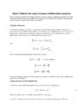
2 Mechanical Systems Spring/mass/damper with md2y/dt2+ cdy/dt + ky = 0, y(0) = y0, y (0) = v0 Solutions depended on parameters Pure oscillation for c = 0 Underdamping when c2< 4km Critical damping when c2= 4km Overdamping when c2> 4km Solution for y/y0depends on ct/m (or tfor c = 0; 2= k/m), km/c2, and mv0/cy0 c2/m2and k/m have dimensions (time) ty/y0v* = 2v* = 1v* = 0v* = -1v* = -2v* = dimensionless initial velocity = v0/ y0 Spring-mass OscillationsNonhomogeneous, Linear, second - order , Differential EquationsOctober 4, 2017ME 501A Seminar in Engineering AnalysisPage 2 Overdamping with 4km/c2 = time ct/mdisplacemenv* = * = * = * = * = * = dimensionless initial velocity = mv0/cy0 Overdamping 4km/c2 = time ct/mdisplacemenv* = * = * = * = * = * = dimensionless initial velocity = mv/cyCritical time ct/my/y0v* = * = * = * = * = * = dimensionless initial velocity = mv0/cy0 Underdamping 4km/c2 = time ct/mdisplacemenv* = * = * = * = * = (-ct/2m)-exp(-ct/2m)

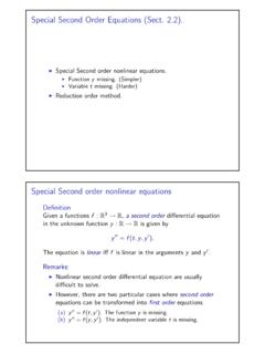
3 V* = dimensionless initial velocity = mv0/cy0 Underdamping 4km/c2 = time ct/mdisplacemenv* = * = * = * = * = (-ct/2m)-exp(-ct/2m)v* = dimensionless initial velocity = mv0/cy012 Alternative Formulations tCtCtCy coscossinsincos tBtAy cossin Proposed alternative with equation from trigonometry for cos(a b) How does this match original equation? Matches if A = C sin and B = C cos This gives A2+ B2= C2sin2 + C2cos2 = C2and A/B = (C sin )/(C cos ) = tan or = tan-1(A/B) = tan-1(v0/y0 )Nonhomogeneous, Linear, second - order , Differential EquationsOctober 4, 2017ME 501A Seminar in Engineering AnalysisPage 313 Nonhomogeneous equations Solution to linear nonhomogeneous second - order equation, y = yH+ yP)()()(22xryxqdxdyxpdxyd 0)()(22 HHHyxqdxdyxpdxyd yHis general solution to corresponding homogenous equation, C1y1+ C2y2 yPis particular solution14 Nonhomogeneous equations II What is first step in solving the general second - order nonhomogeneous ODE?

4 ()()(22xryxqdxdyxpdxyd 0)()(22 HHHyxqdxdyxpdxyd First step is finding yH, which is the general solution to corresponding homogenous equation15 Nonhomogeneous equations III Substitute solution y = yH+ yPinto the nonhomogeneous equation )()()(22xryyxqdxyydxpdxyydPHPHPH )()()()()(2222xryxqyxqdxdyxpdxdyxpdxyddx ydPHPHPH )()()()()(2222xryxqdxdyxpdxydyxqdxdyxpdx ydPPPHHH )()()(22xryxqdxdyxpdxydPPP HomogeneousEquation = 016 Nonhomogeneous equations IV Solve nonhomogeneous equations by first finding homogeneous solution)()()(22xryxqdxdyxpdxydPPP 0)()(22 HHHyxqdxdyxpdxyd Do not solve for C1and C2in homogenous solution yH= C1y1+ C2y2 Solve for yP Apply initial/boundary conditions to y = C1y1+ C2y2+ yPto get C1and C217 Solving Method of undetermined coefficients applies for constant coefficient equation Assume a solution for yPbased on the form of r(x) with constants Process for assuming yPto be described later , if r(x) = x2assume a solution of the form yP= a0+ a1x + a2x2 Substitute proposed solution into the Differential equation for yP Set coefficient sum of like termsin yPto zero Solve for the unknown akcoefficients in yP)(22xrydxdydxydPPP 18 Example.)

5 Solve Assume yP= a0+ a1x + a2x2 Substitute yP, dyP/dx = a1+ 2a2x and d2yP/dx2= 2a2into Differential equation22223xydxdydxydPPP 201221222232xaxaxaaxaa Set coefficient sums of like terms (like powers of x in this example) to zero 2a2+ 3a1+ 2a0= 0 for x0 terms 6a2+ 2a1= 0 for x1 terms 2a2= 1 for x2 terms3 equations for a0, a1, and a2solved on next slideNonhomogeneous, Linear, second - order , Differential EquationsOctober 4, 2017ME 501A Seminar in Engineering AnalysisPage 419 Example: solve22223xydxdydxydPPP 2a2+ 3a1+ 2a0= 0 => a0= -a2-3a1/2 6a2+ 2a1= 0 => a1= -3a2 2a2= 1 => a2= so a1= -3a2= -3/2 a0= -a2-3a1/2 = -1/2 3(-3/2)/2 = 7/4 So yP= a0+ a1x + a2x2= 7/4 3x/2 + x2/2 Check this: yP + 3yP + 2yP= 1+ 3(x 3/2) + 2(7/4 3x/2+ x2/2) = 1 9/2 + 7/2+ x(3 3)+ x2= x2proving solution for yP20 Example: solve22223xydxdydxyd Just found yP= 7/4 3x/2 + x2/2 Characteristic equation for homogenous ODE has two distinct real roots y = yH+ yP= C1e-2x+ C2e-x+ 7/4 3x/2 + x2/2 Find C1and C2from initial conditions such as y(0) = y0and y (0) = v01,22)2(4332422 21 Example: solve22223xydxdydxyd y = C1e-2x+ C2e-x+ 7/4 3x/2 + x2/2 y = -2C1e-2x-C2e-x 3/2 + x y0= C1e0+ C2e0+ 7/4 3(0)/2 + 02/2 y0= C1+ C2+ 7/4 => C2= y0 7/4 C1 v0= 2C1e0 C2e0 3/2 + 0 v0= 2C1 C2 3/2 y0+ v0= C1+ C2+ 7/4 + ( 2C1 C2 3/2) C1= y0 v0 C2= y0 7/4 C1= 2y0+ v0 222 Example.

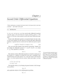
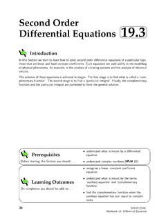
6 Solve22223xydxdydxyd Summary of process to solve nonhomo-geneous ODE with given initial conditions First found yH= C1e-2x+ C2e-x Next found yP= 7/4 3x/2 + x2/2 Wrote y = yH+ yP(including C1and C2) Then used initial conditions on y and dy/dx to find C1= y0 v0 and C2= 2y0+ v0 2 Substitute C1and C2equations into solution for y to get desired result y = ( y0 v0)e-2x+ (2y0+ v0 2)e-x+ 7/4 3x/2 + x2/223 Finding Particular Solution Used for constant coefficient equation y + ay + by = r(x) Solution is y = yP+ yH, where yHis solution of yH + ayH + byH= 0 Postulate a solution for yPfollowing gidelines on next two charts Plug postulated yPsolution into ODE and solve for unknown coefficients Overall coefficients of like terms on both sides of ODE must vanish24 Table of Trial yPSolutionsFor these r(x)Start with this yPr(x) = AeaxyP= Beaxr(x) = AxnyP= a0+ a1x +.

7 + anxnr(x) = Asin xyP= B sin x + C cos xr(x) = Acos xr(x) = Aeaxsin xyP= eax(B sin x + C cos x)r(x) = Aeaxcos xNonhomogeneous, Linear, second - order , Differential EquationsOctober 4, 2017ME 501A Seminar in Engineering AnalysisPage 525 Special Rules If the right-hand-side, r(x) consists of more than one term from the previous table, use a yPthat contains all the corresponding yPterms For r(x) = Acos bx + Cedx, use yP= E sin bx+ F cos bx + Gedx If r(x) is proportional to a solution for the homogenous equation, use yPequal to x times the yPshown in the table For a double root, multiply table yPby x226 Exercise: solve)5cos(22322xydxdydxyd Previous example with new right hand side Keep same initial conditions y(0) = y0and dy/dx(0) = v0 Will have same homogenous solution found previously: yH= C1e-2x+ C2e-x Find new particular solution for 2cos(5x) Use initial conditions on y and dy/dx to find C1and C2 Substitute C1and C2equations into solution for y to get desired result27 Variation of Parameters Background we previously stated the solution to the general first- order linear equation dy/dx + f(x)y = g(x) dxxgeCeydxxfppp)()( Now we derive this solution as an example of variation of parameters Start with solution to homogenous equation.

8 DyH/dx + f(x)yH= 028 Variation of Parameters II Homogenous equation has separable solution found below dxxfpeydxxfydxxfydyyxfdxdypHHHHHH)()(ln) ()( Try a solution to the nonhomogenousequation of the form y(x) = u(x)yH(x) This gives y = u yH+ uyH Substitute this into original equationdy/dx + f(x)y = g(x)29 Variation of Parameters III Rearrange equation to get homogenous Differential equation with yHthat is zero )()()()()()()(xgdxduyxgdxduyyxfdxdyuxguy xfdxdyudxduyxgyxfdxdyHHHHHHH Since we know yH(x), we now have a separable ODE to solve for uas shown on the next chartln 30 Variation of Parameters IV Rearrange final (separable) Differential equation to solve for u by integration CdxyxguyxgdxduxgdxduyHHH)()()( Can we apply this to second - order ?

9 DxxfpueuyySubstitutepH)(CdxxgeeCdxyxgyuy ydxxfdxxfHHH )()()()(Nonhomogeneous, Linear, second - order , Differential EquationsOctober 4, 2017ME 501A Seminar in Engineering AnalysisPage 631 Variation of Parameters V Nonhomogenous and homogenous equations y1(x) and y2(x) are LI homogenous solutions Try solution y = u(x) y1(x) + v(x) y2(x) Two functions but one equation Create another (arbitrary) equation)()()(22xryxqdxdyxpdxyd 0)()(11212 yxqdxdyxpdxyd0)()(22222 yxqdxdyxpdxyd32 Variation of Parameters VI First derivative of y(x) is = u (x) y1(x) + u(x) y1 (x) + v (x) y2(x) + v(x) y2 (x) Pick arbitrary second equation to simplify result: u (x) y1(x) + v (x) y2(x) = 0 This gives y (x) = u(x) y1 (x) + v(x) y2 (x) y = uy1 + u y1 +vy2 + v y2 Substitute results for y, y , and y into the original Differential equation33 Variation of Parameters VIIrdxdydxdvdxdydxduqydxdypdxydvqydxdypd xydu 212222211212 Rearrange to get homogenous ODE equal zero with solutions y1and y2 Homogenous ODEs = zerorvyuyqdxdyvdxdyupdxdydxdvdxydvdxdydx dudxydurqydxdypdxyd )

10 (2121222212122234 Variation of Parameters VIII rdxdvdxdydxdudxdy 21 Two equations in two unknowns Auxiliary equation ODE Result021 dxdvydxduy Multiply first equation by y1, second equation by dy1/dx and subtractrydxdvWdxdvdxdyydxdyy11221 35 Variation of Parameters IXrdxdvdxdydxdudxdy 21 Repeat last chart with change to get equation for du/dx instead of dv/dx Auxiliary equation ODE Result021 dxdvydxduy Multiply first equation by y2, second equation by dy2/dx and subtract first from secondrydxduWdxdudxdyydxdyy21221 36 Variation of Parameters X dxxWxryvdxxWxryu)()()()(12 Integrate du/dx and dv/dx equations Plug into original solution: yP= y1u + y2v Get y = yH+ yPand evaluate constants in yHsolution from initial conditions dxxWxryydxxWxryyvyuyyP)()()()(122121 Nonhomogeneous, Linear, second - order , Differential EquationsOctober 4, 2017ME 501A Seminar in Engineering AnalysisPage 737 Nonhomogenous Summary Undetermined coefficients is simpler approach but is limited Constant coefficient equations Limited set of functions Variation of parameters is more complex, but handles more cases In reality, there are no g)