Transcription of Nonlinear Regression Functions
1 SW Ch 8 1/54/ Nonlinear Regression Functions SW Ch 8 2/54/The TestScore STR relation looks linear (maybe).. SW Ch 8 3/54/But the TestScore Income relation looks SW Ch 8 4/54/ Nonlinear Regression General Ideas If a relation between Y and X is Nonlinear : The effect on Y of a change in X depends on the value of X that is, the marginal effect of X is not constant A linear Regression is mis-specified: the functional form is wrong The estimator of the effect on Y of X is biased: in general it isn t even right on average. The solution is to estimate a Regression function that is Nonlinear in X SW Ch 8 5/54/The general Nonlinear population Regression function Yi = f(X1i, X2i.)
2 , Xki) + ui, i = 1,.., n Assumptions 1. E(ui| X1i, X2i,.., Xki) = 0 (same) 2. (X1i,.., Xki, Yi) are (same) 3. Big outliers are rare (same idea; the precise mathematical condition depends on the specific f) 4. No perfect multicollinearity (same idea; the precise statement depends on the specific f) SW Ch 8 6/54/ Outline 1. Nonlinear (polynomial) Functions of one variable 2. Polynomial Functions of multiple variables: Interactions 3. Application to the California Test Score data set 4. Addendum: Fun with logarithms SW Ch 8 7/54/ Nonlinear (Polynomial) Functions of a One RHS Variable Approximate the population Regression function by a polynomial: Yi = 0 + 1Xi + 22iX +.
3 + rriX + ui This is just the linear multiple Regression model except that the regressors are powers of X! Estimation, hypothesis testing, etc. proceeds as in the multiple Regression model using OLS The coefficients are difficult to interpret, but the Regression function itself is interpretable SW Ch 8 8/54/Example: the TestScore Income relation Incomei = average district income in the ith district (thousands of dollars per capita) Quadratic specification: TestScorei = 0 + 1 Incomei + 2(Incomei)2 + ui Cubic specification: TestScorei = 0 + 1 Incomei + 2(Incomei)2 + 3(Incomei)3 + ui SW Ch 8 9/54/Estimation of the quadratic specification in STATA generate avginc2 = avginc*avginc.
4 Create a new regressor reg testscr avginc avginc2, r; Regression with robust standard errors Number of obs = 420 F( 2, 417) = Prob > F = R-squared = Root MSE = ---------------------------------------- -------------------------------------- | Robust testscr | Coef.
5 Std. Err. t P>|t| [95% Conf. Interval] -------------+-------------------------- -------------------------------------- avginc | .2680941 avginc2 | .0047803 _cons | ---------------------------------------- -------------------------------------- Test the null hypothesis of linearity against the alternative that the Regression function is a SW Ch 8 10/54/Interpreting the estimated Regression function: (a) Plot the predicted values TestScore = + (Incomei)2 ( ) ( ) ( ) SW Ch 8 11/54/Interpreting the estimated Regression function, ctd.
6 (b) Compute effects for different values of X TestScore = + (Incomei)2 ( ) ( ) ( ) Predicted change in TestScore for a change in income from $5,000 per capita to $6,000 per capita: TestScore = + 6 62 ( + 5 52) = SW Ch 8 12/54/ TestScore = + (Incomei)2 Predicted effects for different values of X: Change in Income ($1000 per capita) TestScore from 5 to 6 from 25 to 26 from 45 to 46 The effect of a change in income is greater at low than high income levels (perhaps, a declining marginal benefit of an increase in school budgets?)
7 Caution! What is the effect of a change from 65 to 66? Don t extrapolate outside the range of the data! SW Ch 8 13/54/Estimation of a cubic specification in STATA gen avginc3 = avginc*avginc2; Create the cubic regressor reg testscr avginc avginc2 avginc3, r; Regression with robust standard errors Number of obs = 420 F( 3, 416) = Prob > F = R-squared = Root MSE = ---------------------------------------- -------------------------------------- | Robust testscr | Coef.
8 Std. Err. t P>|t| [95% Conf. Interval] -------------+-------------------------- -------------------------------------- avginc | .7073505 avginc2 | .0289537 avginc3 | .0006855 .0003471 .0013677 _cons | ---------------------------------------- -------------------------------------- SW Ch 8 14/54/Testing the null hypothesis of linearity, against the alternative that the population Regression is quadratic and/or cubic, that is, it is a polynomial of degree up to 3: H0: population coefficients on Income2 and Income3 = 0 H1: at least one of these coefficients is nonzero.
9 Test avginc2 avginc3; Execute the test command after running the Regression ( 1) avginc2 = ( 2) avginc3 = F( 2, 416) = Prob > F = The hypothesis that the population Regression is linear is rejected at the 1% significance level against the alternative that it is a polynomial of degree up to 3. SW Ch 8 15/54/Summary: polynomial Regression Functions Yi = 0 + 1Xi + 2 2iX +..+ rriX + ui Estimation: by OLS after defining new regressors Coefficients have complicated interpretations To interpret the estimated Regression function: o plot predicted values as a function of x o compute predicted Y/ X at different values of x Hypotheses concerning degree r can be tested by t- and F-tests on the appropriate (blocks of) variable(s).
10 Choice of degree r o plot the data; t- and F-tests, check sensitivity of estimated effects; judgment. o Or use model selection criteria (later) SW Ch 8 16/54/ Polynomials in Multiple Variables: Interactions Perhaps a class size reduction is more effective in some circumstances than in Perhaps smaller classes help more if there are many English learners, who need individual attention That is, TestScoreSTR might depend on PctEL More generally, 1YX might depend on X2 How to model such interactions between X1 and X2? We first consider binary X s, then continuous X s SW Ch 8 17/54/(a) Interactions between two binary variables Yi = 0 + 1D1i + 2D2i + ui D1i, D2i are binary 1 is the effect of changing D1=0 to D1=1.