Transcription of Partial Differential Equations in MATLAB 7
1 Partial Differential Equations in MATLAB HowardSpring 2010 Contents1 PDE in One Space Single Equations .. Single Equations with Variable Coefficients .. Systems .. Systems of Equations with Variable Coefficients .. 112 Single PDE in Two Space Elliptic PDE .. Parabolic PDE .. 163 Linear systems in two space Two Equations .. 184 Nonlinear elliptic PDE in two space Single nonlinear elliptic Equations .. 205 General nonlinear systems in two space Parabolic Problems .. 216 Defining more complicated geometries267 About FEMLAB .. Getting Started with FEMLAB .. 271 PDE in One Space DimensionFor initial boundary value Partial differential equationswith timetand a single spatialvariablex, MATLAB has a built-in Single equationsExample , for example, that we would like to solve the heat equationut=uxxu(t,0) = 0, u(t,1) = 1u(0, x) =2x1 +x2.
2 ( ) MATLAB specifies such parabolic PDE in the formc(x, t, u, ux)ut=x m x(xmb(x, t, u, ux))+s(x, t, u, ux),with boundary conditionsp(xl, t, u) +q(xl, t) b(xl, t, u, ux) = 0p(xr, t, u) +q(xr, t) b(xr, t, u, ux) = 0,wherexlrepresents the left endpoint of the boundary andxrrepresents the right endpointof the boundary, and initial conditionu(0, x) =f(x).(Observe that the same functionbappears in both the equation and the boundary condi-tions.) Typically, for clarity, each set of functions will be specified in a separate M-file. Thatis, the functionsc,b, andsassociated with the equation should be specified in one M-file, thefunctionspandqassociated with the boundary conditions in a second M-file (again, keep inmind thatbis the same and only needs to be specified once), and finally theinitial functionf(x) in a third. The commandpdepewill combine these M-files and return a solution to theproblem.
3 In our example, we havec(x, t, u, ux) =1b(x, t, u, ux) =uxs(x, t, u, ux) =0,which we specify in the function (The specificationm= 0 will be made later.)function [c,b,s] = eqn1(x,t,u,DuDx)%EQN1: MATLAB function M-file that specifies%a PDE in time and one space = 1;b = DuDx;s = 0;For our boundary conditions, we havep(0, t, u) =u;q(0, t) = 0p(1, t, u) =u 1;q(1, t) = 0,which we specify in the function [pl,ql,pr,qr] = bc1(xl,ul,xr,ur,t)%BC1: MATLAB function M-file that specifies boundary conditions%for a PDE in time and one space = ul;ql = 0;pr = ur-1;qr = 0;For our initial condition, we havef(x) =2x1 +x2,which we specify in the function value = initial1(x)%INITIAL1: MATLAB function M-file that specifies the initialcondition%for a PDE in time and one space = 2*x/(1+x 2);We are finally ready to solve the PDE withpdepe. In the following script M-file, we choosea grid ofxandtvalues, solve the PDE and create a surface plot of its solution (given inFigure ).
4 %PDE1: MATLAB script M-file that solves and plots%solutions to the PDE stored in = 0;%NOTE: m=0 specifies no symmetry in the problem. Taking%m=1 specifies cylindrical symmetry, while m=2 specifies%spherical the solution meshx = linspace(0,1,20);t = linspace(0,2,10);%Solve the PDEu = pdepe(m,@eqn1,@initial1,@bc1,x,t);%Plot solutionsurf(x,t,u);title( Surface plot of solution. );xlabel( Distance x );ylabel( Time t );Often, we find it useful to plot solutionprofiles, for whichtis fixed, anduis plottedagainstx. The solutionu(t, x) is stored as a matrix indexed by the vector indices example,u(1,5) returns the value ofuat the point (t(1), x(5)). We can plotuinitially(att= 0) with the commandplot(x,u(1,:))(see Figure ).Finally, a quick way to create a movie of the profile s evolution in time is with thefollowing MATLAB xSurface plot of tFigure : Mesh plot for solution to Equation ( ) Profile for t=0xuFigure : Solution Profile att= = plot(x,u(1,:), erase , xor )for k=2:length(t)set(fig, xdata ,x, ydata ,u(k,:))pause(.)
5 5)endIf you try this out, observe how quickly solutions to the heatequation approach their equi-librium configuration. (The equilibrium configuration is the one that ceases to change intime.) Single Equations with Variable CoefficientsThe following example arises in a roundabout way from the theory of detonation the linearconvection diffusionequationut+ (a(x)u)x=uxxu(t, ) =u(t,+ ) = 0u(0, x) =11 + (x 5)2,wherea(x) is defined bya(x) = 3 u(x)2 2 u(x),with u(x) defined implicitly through the relation1 u+ log|1 u u|=x.(The function u(x) is an equilibrium solution to the conservation lawut+ (u3 u2)x=uxx,with u( ) = 1 and u(+ ) = 0. In particular, u(x) is a solution typically referred to as adegenerate viscous shock wave.)Since the equilibrium solution u(x) is defined implicitly in this case, we first write aMATLAB M-file that takes values ofxand returns values u(x).
6 Observe in this M-file thatthe guess forfzero()depends on the value value = degwave(x)%DEGWAVE: MATLAB function M-file that takes a value x%and returns values for a standing wave solution to%ut + (u 3 - u 2)x = uxxguess = .5;if x<-35value = 1;else5if x>2guess = 1/x;elseif x> = .6;elseguess = 1-exp(-2)*exp(x);endvalue = fzero(@f,guess,[],x);endfunction value1 = f(u,x)value1 = (1/u)+log((1-u)/u)-x;The equation is now stored [c,b,s] = deglin(x,t,u,DuDx)%EQN1: MATLAB function M-file that specifies%a PDE in time and one space = 1;b = DuDx - (3*degwave(x) 2 - 2*degwave(x))*u;s = 0;In this case, the boundary conditions are at . Since MATLAB only understands finitedomains, we will approximate these conditions by settingu(t, 50) =u(t,50) = 0. Observethat at least initially this is a good approximation sinceu0( 50) = 4 andu0(+50) = 4. The boundary conditions are stored in the MATLAB [pl,ql,pr,qr] = degbc(xl,ul,xr,ur,t)%BC1: MATLAB function M-file that specifies boundary conditions%for a PDE in time and one space = ul;ql = 0;pr = ur;qr = 0;The initial condition is specified value = deginit(x)%DEGINIT: MATLAB function M-file that specifies the initial condition%for a PDE in time and one space = 1/(1+(x-5) 2);Finally, we solve and plot this equation : MATLAB script M-file that solves and plots%solutions to the PDE stored in a superfluous warning:clear h;warning off MATLAB :fzero:UndeterminedSyntax6m = 0;%%Define the solution meshx = linspace(-50,50,200);t = linspace(0,10,100);%u = pdepe(m,@deglin,@deginit,@degbc,x,t);%Cr eate profile movieflag = 1;while flag==1answer = input( Finished iteration.)
7 View plot (y/n) , s )if isequal(answer, y )figure(2)fig = plot(x,u(1,:), erase , xor )for k=2:length(t)set(fig, xdata ,x, ydata ,u(k,:))pause(.4)endelseflag = 0;endendThe linewarning off MATLAB :fzero:UndeterminedSyntaxsimply turns off an error messageMATLAB issued every time it calledfzero(). Observe that the option to view a movie ofthe solution s time evolution is given inside a for-loop so that it can be watched repeatedlywithout re-running the file. The initial and final configurations of the solution to this exampleare given in Figures and SystemsWe next consider a system of two Partial differential Equations , though still in time and onespace the nonlinear system of Partial differential equationsu1t=u1xx+u1(1 u1 u2)u2t=u2xx+u2(1 u1 u2),u1x(t,0) = 0;u1(t,1) = 1u2(t,0) = 0;u2x(t,1) = 0,u1(0, x) =x2u2(0, x) =x(x 2).( )(This is a non-dimensionalized form of a PDE model for two competing populations.
8 Aswith solving ODE in MATLAB , the basic syntax for solving systems is the same as for7 50 40 30 20 Functionxu(0,x)Figure : Initial Condition for Example 50 40 30 20 Profilexu(10,x)Figure : Final profile for Example single Equations , where each scalar is simply replaced by an analogous vector. Inparticular, MATLAB specifies a system ofnPDE asc1(x, t, u, ux)u1t=x m x(xmb1(x, t, u, ux))+s1(x, t, u, ux)c2(x, t, u, ux)u2t=x m x(xmb2(x, t, u, ux))+s2(x, t, u, ux)..cn(x, t, u, ux)unt=x m x(xmbn(x, t, u, ux))+sn(x, t, u, ux),(observe that the functionsck,bk, andskcan depend on all components ofuandux) withboundary conditionsp1(xl, t, u) +q1(xl, t) b1(xl, t, u, ux) =0p1(xr, t, u) +q1(xr, t) b1(xr, t, u, ux) =0p2(xl, t, u) +q2(xl, t) b2(xl, t, u, ux) =0p2(xr, t, u) +q2(xr, t) b2(xr, t, u, ux) = (xl, t, u) +qn(xl, t) bn(xl, t, u, ux) =0pn(xr, t, u) +qn(xr, t) bn(xr, t, u, ux) =0,and initial conditionsu1(0, x) =f1(x)u2(0, x) =f2(x).
9 Un(0, x) =fn(x).In our example equation, we havec=(c1c2)=(11);b=(b1b2)=(u1xu2x);s=(s 1s2)=(u1(1 u1 u2)u2(1 u1 u2)),which we specify with the MATLAB [c,b,s] = eqn2(x,t,u,DuDx)%EQN2: MATLAB M-file that contains the coefficents for%a system of two PDE in time and one space = [1; 1];b = [1; 1] .* DuDx;s = [u(1)*(1-u(1)-u(2)); u(2)*(1-u(1)-u(2))];9 For our boundary conditions, we havep(0, t, u) =(p1p2)=(0u2);q(0, t) =(q1q2)=(10)p(1, t, u) =(p1p2)=(u1 10);q(1, t) =(q1q2)=(01)which we specify in the function [pl,ql,pr,qr] = bc2(xl,ul,xr,ur,t)%BC2: MATLAB function M-file that defines boundary conditions%for a system of two PDE in time and one space = [0; ul(2)];ql = [1; 0];pr = [ur(1)-1; 0];qr = [0; 1];For our initial conditions, we haveu1(0, x) =x2u2(0, x) =x(x 2),which we specify in the function value = initial2(x);%INITIAL2: MATLAB function M-file that defines initial conditions%for a system of two PDE in time and one space = [x 2; x*(x-2)];We solve equation ( ) and plot its solutions (see Figure ).
10 %PDE2: MATLAB script M-file that solves the PDE%stored in , , and = 0;x = linspace(0,1,10);t = linspace(0,1,10);sol = pdepe(m,@eqn2,@initial2,@bc2,x,t);u1 = sol(:,:,1);u2 = sol(:,:,2);subplot(2,1,1)surf(x,t,u1);ti tle( u1(x,t) );xlabel( Distance x );ylabel( Time t );subplot(2,1,2)surf(x,t,u2);title( u2(x,t) );xlabel( Distance x );ylabel( Time t ); xu1(x,t)Time 1 xu2(x,t)Time tFigure : Mesh plot of solutions for Example Systems of Equations with Variable CoefficientsWe next consider a system analogue to Example the system of convection diffusion equationsu1t 2u1x u2x=u1xxu2t u1x 2u2x (3 u1(x)2u1) =u2xxu1(t, ) =u1(t,+ ) = 0u2(t, ) =u2(t,+ ) = 0u1(0, x) =e (x 5)2u2(0, x) =e (x+5)2,where u1(x) is the first component in the solution of the boundary value ODE system u1x= 2( u1+ 2) u2 u2x= ( u1+ 2) 2 u2 ( u31+ 8) u1( ) = 2; u1(+ ) = 1 u2( ) = 0; u2(+ ) = this case, the vector function u(x) = ( u1(x), u2(x))tris a degenerate viscous shock solutionto the conservation lawu1t 2u1x u2x=u1xxu2t u1x 2u2x (u31)x= of the main obstacles of this example is that it is prohibitively difficult to develop evenan implicit representation for u(x).